2.2: Teoría de Orbitales Moleculares (MO) (Revisión)

Última actualización
Guardar como PDF

Page ID: 76707

\( \newcommand{\vecs}[1]{\overset { \scriptstyle \rightharpoonup} {\mathbf{#1}} } \) \( \newcommand{\vecd}[1]{\overset{-\!-\!\rightharpoonup}{\vphantom{a}\smash {#1}}} \)\(\newcommand{\id}{\mathrm{id}}\) \( \newcommand{\Span}{\mathrm{span}}\) \( \newcommand{\kernel}{\mathrm{null}\,}\) \( \newcommand{\range}{\mathrm{range}\,}\) \( \newcommand{\RealPart}{\mathrm{Re}}\) \( \newcommand{\ImaginaryPart}{\mathrm{Im}}\) \( \newcommand{\Argument}{\mathrm{Arg}}\) \( \newcommand{\norm}[1]{\| #1 \|}\) \( \newcommand{\inner}[2]{\langle #1, #2 \rangle}\) \( \newcommand{\Span}{\mathrm{span}}\) \(\newcommand{\id}{\mathrm{id}}\) \( \newcommand{\Span}{\mathrm{span}}\) \( \newcommand{\kernel}{\mathrm{null}\,}\) \( \newcommand{\range}{\mathrm{range}\,}\) \( \newcommand{\RealPart}{\mathrm{Re}}\) \( \newcommand{\ImaginaryPart}{\mathrm{Im}}\) \( \newcommand{\Argument}{\mathrm{Arg}}\) \( \newcommand{\norm}[1]{\| #1 \|}\) \( \newcommand{\inner}[2]{\langle #1, #2 \rangle}\) \( \newcommand{\Span}{\mathrm{span}}\)\(\newcommand{\AA}{\unicode[.8,0]{x212B}}\)

Objetivo de aprendizaje

escribir e interpretar diagramas orbitales moleculares (MO)

Visión general

La teoría orbital molecular (MO) describe el comportamiento de los electrones en una molécula en términos de combinaciones de las funciones de onda atómica. Los orbitales moleculares resultantes pueden extenderse sobre todos los átomos de la molécula. Los orbitales moleculares de unión están formados por combinaciones en fase de funciones de ondas atómicas, y los electrones en estos orbitales estabilizan una molécula. Los orbitales moleculares antiadherentes resultan de combinaciones desfasadas y los electrones en estos orbitales hacen que una molécula sea menos estable.

La teoría orbital molecular describe la distribución de electrones en moléculas de la misma manera que se describe la distribución de electrones en átomos usando orbitales atómicos. Utilizando la mecánica cuántica, el comportamiento de un electrón en una molécula todavía se describe mediante una función de onda, ψ, análoga al comportamiento en un átomo. Al igual que los electrones alrededor de átomos aislados, los electrones alrededor de los átomos en las moléculas se limitan a energías discretas (cuantificadas). La región del espacio en la que es probable que se encuentre un electrón de valencia en una molécula se denomina orbital molecular (ψ ²). Al igual que un orbital atómico, un orbital molecular está lleno cuando contiene dos electrones con espín opuesto.

Consideraremos los orbitales moleculares en moléculas compuestas por dos átomos idénticos (H ₂ o Cl ₂, por ejemplo). Tales moléculas se llaman moléculas diatómicas homonucleares. En estas moléculas diatómicas ocurren varios tipos de orbitales moleculares.

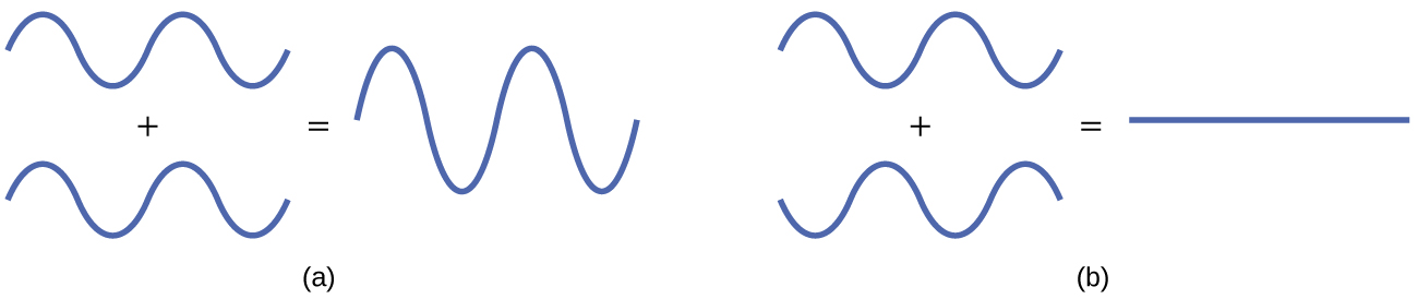
El proceso matemático de combinar orbitales atómicos para generar orbitales moleculares se denomina combinación lineal de orbitales atómicos (LCAO). La función de onda describe las propiedades onduladas de un electrón. Los orbitales moleculares son combinaciones de funciones de ondas orbitales atómicas. La combinación de ondas puede conducir a interferencia constructiva, en la que los picos se alinean con picos, o interferencia destructiva, en la que los picos se alinean con valles (Figura\(\PageIndex{2}\)). En los orbitales, las ondas son tridimensionales, y se combinan con ondas en fase produciendo regiones con una mayor probabilidad de densidad electrónica y ondas fuera de fase que producen nodos, o regiones sin densidad electrónica.

Se muestran y etiquetan un par de diagramas, “a” y “b”. El diagrama a muestra dos ondas idénticas con dos crestas y dos canales. Se dibujan uno encima del otro con un signo más en el medio y un signo igual a la derecha. A la derecha del signo igual se encuentra una ola mucho más alta con un mismo número de abrevaderos y crestas. El diagrama b muestra dos ondas con dos crestas y dos valles, pero son imágenes especulares entre sí giradas sobre un eje horizontal. Se dibujan uno encima del otro con un signo más en el medio y un signo igual a la derecha. A la derecha del signo igual hay una línea plana. — Figura\(\PageIndex{2}\): (a) Cuando las ondas en fase se combinan, la interferencia constructiva produce una onda con mayor amplitud. (b) Cuando las ondas fuera de fase se combinan, la interferencia destructiva produce una onda con menor (o ninguna) amplitud.

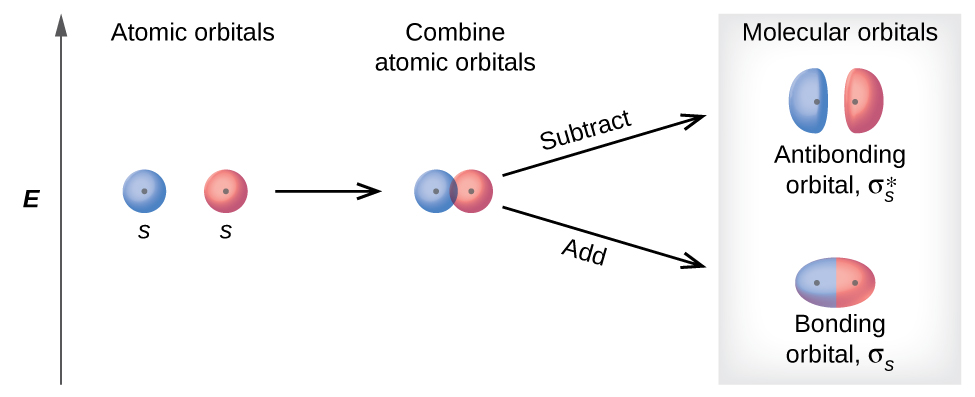
Hay dos tipos de orbitales moleculares que se pueden formar a partir de la superposición de dos orbitales atómicos en átomos adyacentes. Los dos tipos se ilustran en la Figura 8.4.3. La combinación en fase produce un orbital molecular σ _s de menor energía (leído como “sigma-s”) en el que la mayor parte de la densidad de electrones se encuentra directamente entre los núcleos. La adición fuera de fase (que también se puede considerar como restando las funciones de onda) produce un orbital molecular de mayor energía\(σ^∗_s\) m olecular (leído como “sigma-s-estrella”) orbital molecular en el que hay un nodo entre los núcleos. El asterisco significa que el orbital es un orbital antiadherentes. Los electrones en un orbital σ _s son atraídos por ambos núcleos al mismo tiempo y son más estables (de menor energía) de lo que serían en los átomos aislados. Agregar electrones a estos orbitales crea una fuerza que mantiene unidos los dos núcleos, por lo que llamamos a estos orbitales que unen orbitales. Los electrones en los\(σ^∗_s\) orbitales se encuentran muy lejos de la región entre los dos núcleos. La fuerza de atracción entre los núcleos y estos electrones separa los dos núcleos. De ahí que estos orbitales se llamen orbitales antiadherentes. Los electrones llenan el orbital de enlace de menor energía antes que el orbital antienlace de mayor energía, así como llenan orbitales atómicos de menor energía antes de llenar orbitales atómicos de mayor energía.

Se muestra un diagrama que representa una flecha vertical orientada hacia arriba que se encuentra a la izquierda de todas las demás partes del diagrama y está etiquetada como “E.” A la derecha inmediata del punto medio de la flecha hay dos círculos etiquetados cada uno con un signo positivo, la letra S, y la frase, “Orbitales atómicos”. A estos les sigue una flecha horizontal orientada hacia la derecha que apunta a los mismos dos círculos etiquetados con signos más, pero ahora se tocan y se etiquetan, “Combinar orbitales atómicos”. Dos flechas orientadas hacia la derecha conducen a la última parte del diagrama, una orientada hacia arriba y otra hacia abajo. La flecha superior está etiquetada como “Restar” y apunta a dos óvalos oblongos etiquetados con signos más, y la frase “Orbitales antiunión sigma subíndice s asterisco superíndice”. La flecha inferior está etiquetada, “Agregar”, y apunta a un óvalo alargado con dos signos más que se etiqueta, “Vinculación de subíndice sigma orbital s.” El encabezamiento de la última sección del diagrama son las palabras, “Orbitales moleculares”. — Figura\(\PageIndex{3}\): Los orbitales moleculares sigma (σ) y sigma-star (σ*) están formados por la combinación de orbitales atómicos de dos s. Los signos más (+) indican la ubicación de los núcleos.

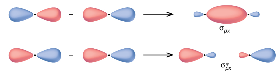
En los orbitales p, la función de onda da lugar a dos lóbulos con fases opuestas, análogas a como una onda bidimensional tiene ambas partes por encima y por debajo del promedio. Indicamos las fases sombreando los lóbulos orbitales de diferentes colores. Cuando los lóbulos orbitales de la misma fase se superponen, la interferencia de ondas constructivas aumenta la densidad de electrones. Cuando las regiones de fase opuesta se superponen, la interferencia de onda destructiva disminuye la densidad de electrones y crea nodos. Cuando los orbitales p se superponen de extremo a extremo, crean orbitales σ y σ* (Figura\(\PageIndex{4}\)). Si dos átomos están ubicados a lo largo del eje x en un sistema de coordenadas cartesianas, los dos orbitales p _x se superponen de extremo a extremo y forman σ _px\(σ^∗_{px}\) (enlace) y (antienlace) (leer como “sigma-p-x” y “estrella sigma-p-x”, respectivamente). Al igual que con el solapamiento s-orbital, el asterisco indica el orbital con un nodo entre los núcleos, que es un orbital antienlace de mayor energía.

Se muestran dos filas horizontales de diagramas. El diagrama superior muestra dos orbitales en forma de cacahuete de igual tamaño con un signo más entre ellos conectados a un diagrama orbital fusionado por una flecha orientada hacia la derecha. El diagrama fusionado tiene un óvalo mucho más grande en el centro y orbitales ovulares mucho más pequeños en el borde. Se etiqueta, “sigma subíndice p x”. El diagrama inferior muestra dos orbitales en forma de cacahuete de igual tamaño con un signo más entre ellos conectados a un diagrama orbital dividido por una flecha orientada hacia la derecha. El diagrama dividido tiene un óvalo mucho más grande en los extremos exteriores y orbitales ovulares mucho más pequeños en los bordes internos. Se etiqueta, “sigma subíndice p x superíndice asterisco”. — Figura\(\PageIndex{4}\): La combinación de funciones de onda de dos orbitales p atómicos a lo largo del eje internuclear crea dos orbitales moleculares, σ _p y\(σ^∗_p\).

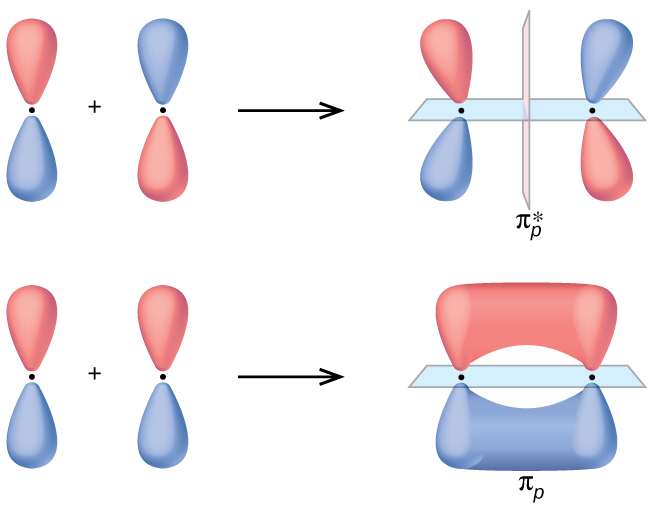
El solapamiento lado a lado de dos orbitales p da lugar a un orbital molecular de enlace pi (π) y un orbital molecular antienlace π*, como se muestra en la Figura\(\PageIndex{5}\). En la teoría de los enlaces de valencia, describimos los enlaces π como que contienen un plano nodal que contiene el eje internuclear y perpendicular a los lóbulos de los orbitales p, con densidad electrónica a ambos lados del nodo. En la teoría orbital molecular, describimos el orbital π con esta misma forma, y existe un enlace π cuando este orbital contiene electrones. Los electrones en este orbital interactúan con ambos núcleos y ayudan a mantener los dos átomos juntos, convirtiéndolo en un orbital de enlace. Para la combinación fuera de fase, se crean dos planos nodales, uno a lo largo del eje internuclear y uno perpendicular entre los núcleos.

Se muestran dos filas horizontales de diagramas. Los diagramas superior e inferior comienzan con dos orbitales verticales en forma de cacahuete con un signo más en el medio seguido de una flecha orientada hacia la derecha. El diagrama superior muestra los mismos orbitales verticales de cacahuete doblándose ligeramente alejándose entre sí y separados por una línea punteada. Se etiqueta, “pi subíndice p superíndice asterisco”. El diagrama inferior muestra el solapamiento horizontal de los dos orbitales y se etiqueta, “pi subíndice p.” — Figura\(\PageIndex{5}\): El solapamiento lado a lado de cada dos orbitales p da como resultado la formación de dos orbitales moleculares π. La combinación de los orbitales fuera de fase da como resultado un orbital molecular antienlace con dos nodos. Uno contiene el eje internuclear, y otro es perpendicular al eje. La combinación de los orbitales en fase da como resultado un orbital de unión. Hay un nodo (plano azul) que contiene el eje internuclear con los dos lóbulos de la órbita ubicados por encima y por debajo de este nodo.

En los orbitales moleculares de las moléculas diatómicas, cada átomo también tiene dos conjuntos de orbitales p orientados lado a lado (p _y p _z), por lo que estos cuatro orbitales atómicos se combinan por pares para crear dos orbitales π y dos orbitales π*. Los π _py y\(π^∗_{py}\) los orbitales están orientados en ángulo recto con el π _pz y\(π^∗_{pz}\) los orbitales. Excepto por su orientación, los orbitales π _py y π _pz son idénticos y tienen la misma energía; son orbitales degenerados. Los orbitales\(π^∗_{py}\) y\(π^∗_{pz}\) antiadherentes también son degenerados e idénticos excepto por su orientación. Un total de seis orbitales moleculares resulta de la combinación de los seis orbitales p atómicos en dos átomos: σ _px y\(σ^∗_{px}\), π _py y\(π^∗_{py}\), π _pz y\(π^∗_{pz}\).

Ejemplo\(\PageIndex{1}\)

Orbitales oleculares M Predecir qué tipo (si existe) de orbital molecular resultaría de sumar las funciones de onda para que cada par de orbitales mostrara solapamiento. Los orbitales son todos similares en energía.

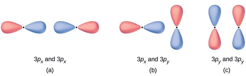
Solución

Esta es una combinación en fase, dando como resultado un orbital σ _{3 p}
Esto no dará como resultado un nuevo orbital porque el componente en fase (inferior) y el componente fuera de fase (arriba) se cancelan. Solo se pueden combinar orbitales con la alineación correcta.
Esta es una combinación fuera de fase, lo que resulta en una
- Paul Flowers (University of North Carolina - Pembroke), Klaus Theopold (University of Delaware) and Richard Langley (Stephen F. Austin State University) with contributing authors. Textbook content produced by OpenStax College is licensed under a Creative Commons Attribution License 4.0 license. Download for free at http://cnx.org/contents/85abf193-2bd...a7ac8df6@9.110).
\(π^∗_{3p}\) orbital.

Exercise \(\PageIndex{1}\)

Label the molecular orbital shown as σ or π, bonding or antibonding and indicate where the node occurs.

Two orbitals are shown lying end-to-end. Each has one enlarged and one small side. The small sides are facing one another

Answer: The orbital is located along the internuclear axis, so it is a σ orbital. There is a node bisecting the internuclear axis, so it is an antibonding orbital.

Molecular Orbital Energy Diagrams

The relative energy levels of atomic and molecular orbitals are typically shown in a molecular orbital diagram (Figure \(\PageIndex{7}\)). For a diatomic molecule, the atomic orbitals of one atom are shown on the left, and those of the other atom are shown on the right. Each horizontal line represents one orbital that can hold two electrons. The molecular orbitals formed by the combination of the atomic orbitals are shown in the center. Dashed lines show which of the atomic orbitals combine to form the molecular orbitals. For each pair of atomic orbitals that combine, one lower-energy (bonding) molecular orbital and one higher-energy (antibonding) orbital result. Thus we can see that combining the six 2p atomic orbitals results in three bonding orbitals (one σ and two π) and three antibonding orbitals (one σ* and two π*).

A diagram is shown that has an upward-facing vertical arrow running along the left side labeled, “E.” At the bottom center of the diagram is a horizontal line labeled, “sigma subscript 2 s,” that has two vertical half arrows drawn on it, one facing up and one facing down. This line is connected to the right and left by upward-facing, dotted lines to two more horizontal lines, each labeled, “2 s.” The line on the left has two vertical half arrows drawn on it, one facing up and one facing down while the line of the right has one half arrow facing up drawn on it. These two lines are connected by upward-facing dotted lines to another line in the center of the diagram, but further up from the first. It is labeled, “sigma subscript 2 s superscript asterisk.” This horizontal line has one upward-facing vertical half-arrow drawn on it. Moving farther up the center of the diagram is a long horizontal line labeled, “sigma subscript 2 p subscript x,” which lies below two horizontal lines. These two horizontal lines lie side-by-side, and labeled, “pi subscript 2 p subscript y,” and, “pi subscript 2 p subscript z.” Both the bottom and top lines are connected to the right and left by upward-facing, dotted lines to three more horizontal lines, each labeled, “2 p.” These sets of lines are connected by upward-facing dotted lines to another single line and then pair of double lines in the center of the diagram, but farther up from the lower lines. They are labeled, “sigma subscript 2 p subscript x superscript asterisk,” and, ““pi subscript 2 p subscript y superscript asterisk,” and, “pi subscript 2 p subscript z superscript asterisk,” respectively. The left and right sides of the diagram have headers that read, ”Atomic orbitals,” while the center is header reads “Molecular orbitals”. — Figure \(\PageIndex{7}\): This is the molecular orbital diagram for the homonuclear diatomic *\(\ce{Be2+}\),* *showing the molecular orbitals of the valence shell only. The molecular orbitals are filled in the same manner as atomic orbitals, using the Aufbau principle and Hund’s rule.*

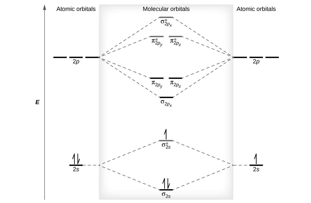
We predict the distribution of electrons in these molecular orbitals by filling the orbitals in the same way that we fill atomic orbitals, by the Aufbau principle. Lower-energy orbitals fill first, electrons spread out among degenerate orbitals before pairing, and each orbital can hold a maximum of two electrons with opposite spins (Figure \(\PageIndex{7}\)). Just as we write electron configurations for atoms, we can write the molecular electronic configuration by listing the orbitals with superscripts indicating the number of electrons present. For clarity, we place parentheses around molecular orbitals with the same energy. In this case, each orbital is at a different energy, so parentheses separate each orbital. Thus we would expect a diatomic molecule or ion containing seven electrons (such as \(\ce{Be2+}\)) would have the molecular electron configuration \((σ_{1s})^2(σ^∗_{1s})^2(σ_{2s})^2(σ^∗_{2s})^1\). It is common to omit the core electrons from molecular orbital diagrams and configurations and include only the valence electrons.

Bond Order

The filled molecular orbital diagram shows the number of electrons in both bonding and antibonding molecular orbitals. The net contribution of the electrons to the bond strength of a molecule is identified by determining the bond order that results from the filling of the molecular orbitals by electrons.

When using Lewis structures to describe the distribution of electrons in molecules, we define bond order as the number of bonding pairs of electrons between two atoms. Thus a single bond has a bond order of 1, a double bond has a bond order of 2, and a triple bond has a bond order of 3. We define bond order differently when we use the molecular orbital description of the distribution of electrons, but the resulting bond order is usually the same. The MO technique is more accurate and can handle cases when the Lewis structure method fails, but both methods describe the same phenomenon.

In the molecular orbital model, an electron contributes to a bonding interaction if it occupies a bonding orbital and it contributes to an antibonding interaction if it occupies an antibonding orbital. The bond order is calculated by subtracting the destabilizing (antibonding) electrons from the stabilizing (bonding) electrons. Since a bond consists of two electrons, we divide by two to get the bond order. We can determine bond order with the following equation:

\[\textrm{bond order}=\dfrac{(\textrm{number of bonding electrons})−(\textrm{number of antibonding electrons})}{2}\]

The order of a covalent bond is a guide to its strength; a bond between two given atoms becomes stronger as the bond order increases. If the distribution of electrons in the molecular orbitals between two atoms is such that the resulting bond would have a bond order of zero, a stable bond does not form. We next look at some specific examples of MO diagrams and bond orders.

Bonding in Diatomic Molecules

A dihydrogen molecule (H₂) forms from two hydrogen atoms. When the atomic orbitals of the two atoms combine, the electrons occupy the molecular orbital of lowest energy, the σ_1s bonding orbital. A dihydrogen molecule, H₂, readily forms because the energy of a H₂ molecule is lower than that of two H atoms. The σ_1s orbital that contains both electrons is lower in energy than either of the two 1s atomic orbitals.

A molecular orbital can hold two electrons, so both electrons in the H₂ molecule are in the σ_1s bonding orbital; the electron configuration is \((σ_{1s})^2\). We represent this configuration by a molecular orbital energy diagram (Figure \(\PageIndex{8}\)) in which a single upward arrow indicates one electron in an orbital, and two (upward and downward) arrows indicate two electrons of opposite spin.

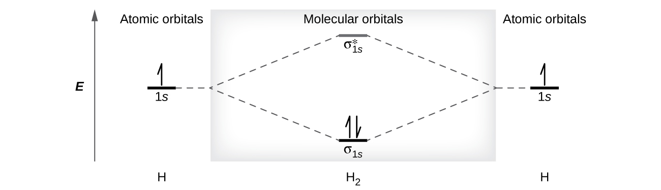
A dihydrogen molecule contains two bonding electrons and no antibonding electrons so we have

\[\ce{bond\: order\: in\: H2}=\dfrac{(2−0)}{2}=1\]

Because the bond order for the H–H bond is equal to 1, the bond is a single bond.

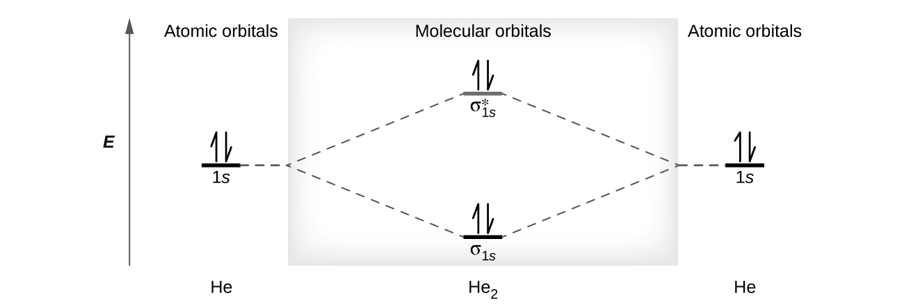
A helium atom has two electrons, both of which are in its 1s orbital. Two helium atoms do not combine to form a dihelium molecule, He₂, with four electrons, because the stabilizing effect of the two electrons in the lower-energy bonding orbital would be offset by the destabilizing effect of the two electrons in the higher-energy antibonding molecular orbital. We would write the hypothetical electron configuration of He₂ as \((σ_{1s})^2(σ^∗_{1s})^2\) as in Figure \(\PageIndex{9}\) . The net energy change would be zero, so there is no driving force for helium atoms to form the diatomic molecule. In fact, helium exists as discrete atoms rather than as diatomic molecules. The bond order in a hypothetical dihelium molecule would be zero.

\[\ce{bond\: order\: in\: He2}=\dfrac{(2−2)}{2}=0\]

A bond order of zero indicates that no bond is formed between two atoms.

Contributors and Attributions

C2−