6.11: Teorema de Ampère

En la Sección 1.9 se introdujo el teorema de Gauss, que es que el componente normal total del\(D\) flujo a través de una superficie cerrada es igual a la carga encerrada dentro de esa superficie. El teorema de Gauss es una consecuencia de la ley de Coulomb, en la que el campo eléctrico de una fuente puntual cae inversamente como el cuadrado de la distancia. Encontramos que el teorema de Gauss fue sorprendentemente útil ya que nos permitió escribir casi de inmediato expresiones para el campo eléctrico en las proximidades de diversas formas de cuerpos cargados sin pasar por mucho cálculo.

¿Existe quizás un teorema similar relacionado con el campo magnético alrededor de un conductor portador de corriente que nos permita calcular el campo magnético en sus proximidades sin pasar por mucho cálculo? De hecho hay, y se llama Teorema de Ampère.

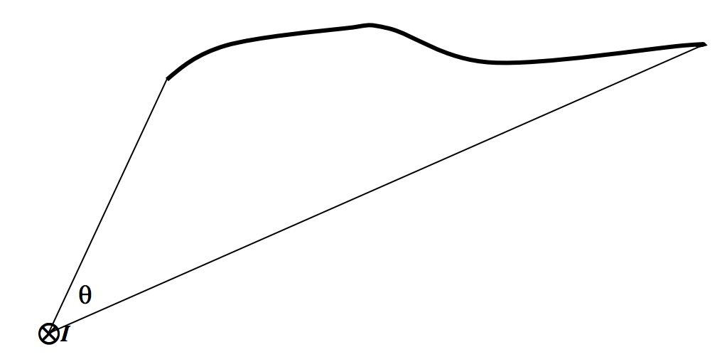
\(\text{FIGURE VI.9}\)

En Figura se supone que\(\text{VI.9}\) hay una corriente que\(I\) viene hacia ti en medio del círculo. He dibujado una de las líneas del campo magnético, una línea discontinua de radio\(r\). La fuerza del campo ahí está\(H = I/(2\pi r)\). También he dibujado una pequeña longitud elemental\(ds\) en la circunferencia del círculo. La línea integral del campo alrededor del círculo es solo\(H\) multiplicada por la circunferencia del círculo. Es decir, la línea integral del campo alrededor del círculo es justa\(I\). Tenga en cuenta que esto es independiente del radio del círculo. A mayores distancias de la corriente, el campo cae como\(1/r\), pero la circunferencia del círculo aumenta a medida que\(r\), por lo que el producto de los dos (la línea integral) es independiente de\(r\).

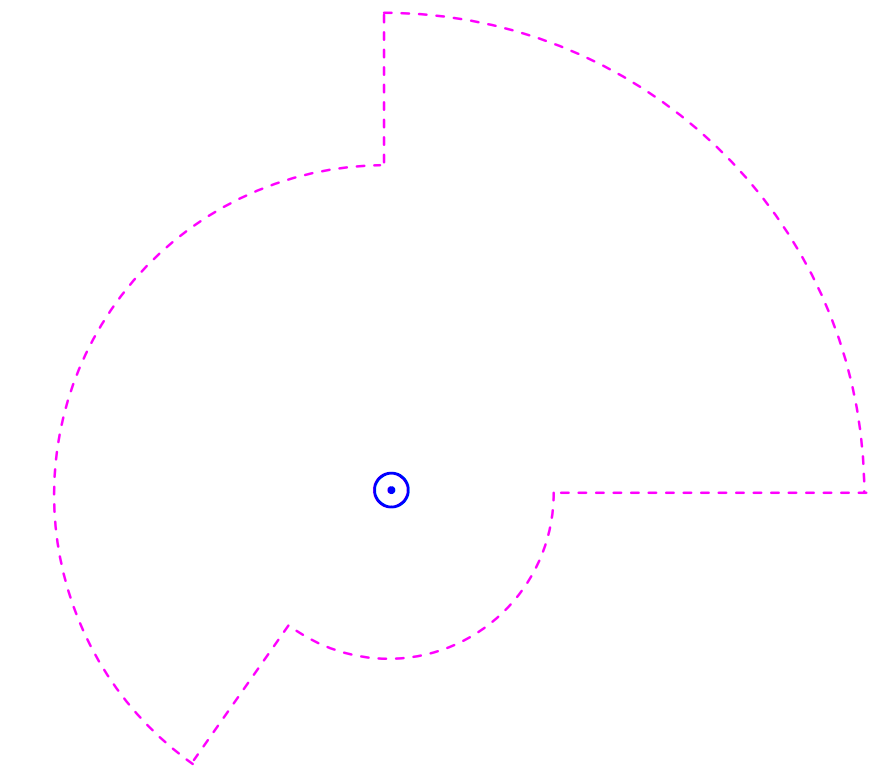
\(\text{FIGURE VI.10}\)

En consecuencia, si calculo la línea integral alrededor de un circuito como el que se muestra en la Figura\(\text{VI.10}\), seguirá llegando a justo\(I\). Efectivamente no importa cuál sea la forma del camino. La línea integral es\(\int \textbf{H}\cdot \textbf{ds}\). El campo\(\textbf{H}\) en algún punto es perpendicular a la línea que une la corriente al punto, y el vector\(\textbf{ds}\) se dirige a lo largo de la trayectoria de integración, y\(\textbf{H}\cdot \textbf{ds}\) es igual a\(H\) veces el componente de a\(\textbf{ds}\) lo largo de la dirección de\(\textbf{H}\), de modo que, independientemente de la longitud y forma del camino de integración:

La integral de línea del campo\(\textbf{H}\) alrededor de cualquier camino cerrado es igual a la corriente encerrada por ese camino.

Este es el teorema de Ampère.

Entonces ahora volvamos a hacer el solenoide infinito. Calculemos la línea integral alrededor de la trayectoria rectangular de amperios que se muestra en la Figura\(\text{VI.11}\). No hay contribución a la línea integral a lo largo de los lados verticales del rectángulo porque estos lados son perpendiculares al campo, y no hay contribución desde el lado superior del rectángulo, ya que el campo hay cero (si el solenoide es infinito). La única contribución a la integral de línea es a lo largo del lado inferior del rectángulo, y la integral de línea hay justo\(Hl\), donde\(l\) está la longitud del rectángulo. Si el número de vueltas de cable por unidad de longitud a lo largo del solenoide es\(n\), habrá\(nl\) vueltas encerradas por el rectángulo, y de ahí la corriente encerrada por el rectángulo es\(nlI\), donde\(I\) está la corriente en el cable. Por lo tanto por el teorema de Ampère\(Hl = nlI\),\(H = nI\), y así, que es lo que deducimos antes bastante más laboriosamente. Aquí\(H\) está la intensidad del campo en la posición del lado inferior del rectángulo; pero podemos colocar el rectángulo a cualquier altura, así vemos que el campo está en\(nI\) cualquier parte dentro del solenoide. Es decir, el campo dentro de un solenoide infinito es uniforme.

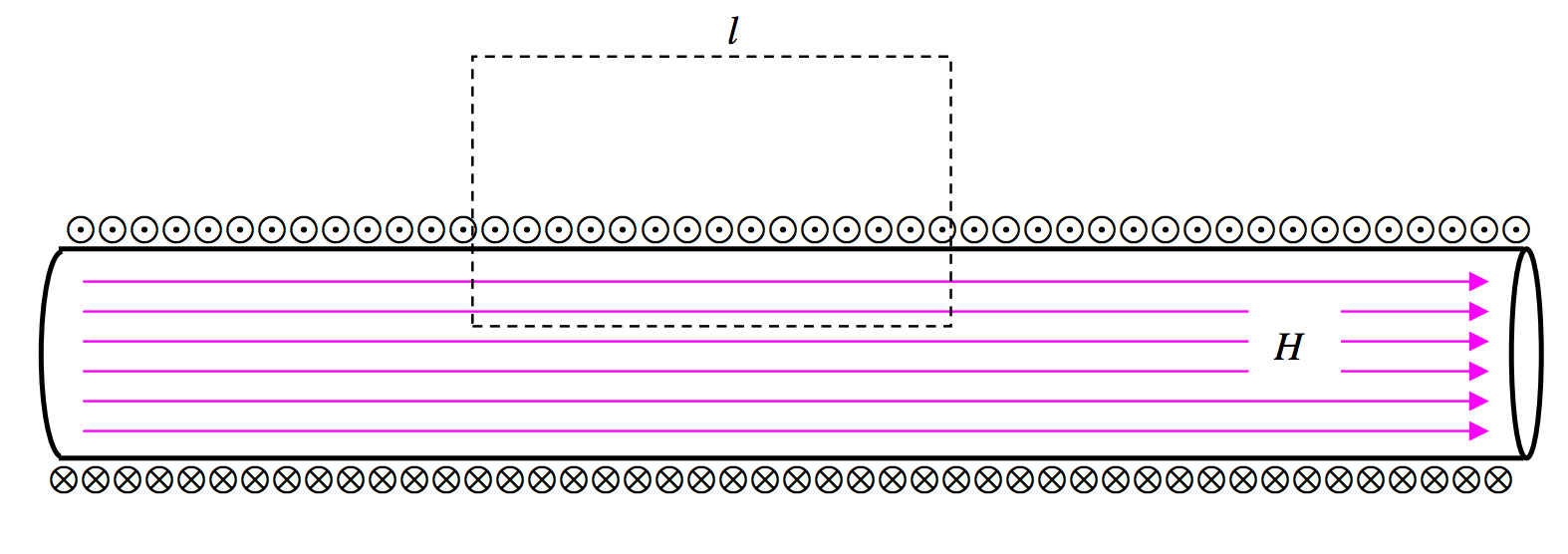
\(\text{FIGURE VI.11}\)

Quizás valga la pena señalar que el teorema de Gauss es una consecuencia de la disminución cuadrada inversa del campo eléctrico con la distancia desde una carga puntual, y el teorema de Ampère es una consecuencia de la disminución inversa de la primera potencia del campo magnético con la distancia de una corriente de línea.

desde el eje,\(r < a\)?

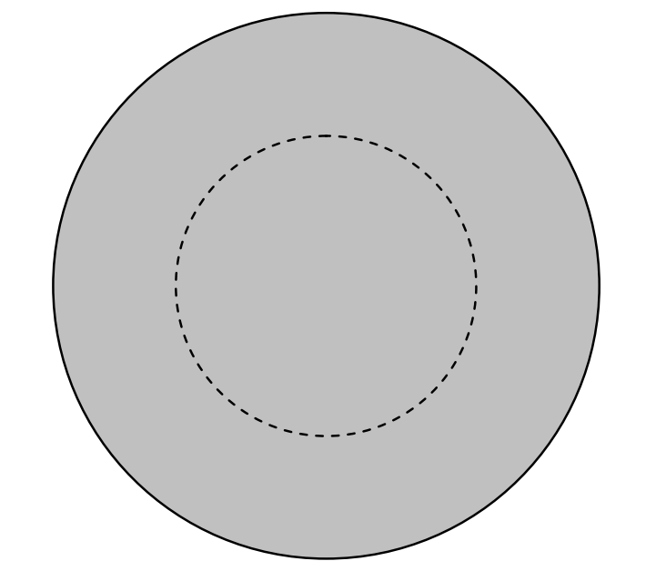
\(\text{FIGURE VI.15}\)

Figure \(\text{VI.15}\) shows the cross-section of the rod, and I have drawn an amperian circle of radius \(r\). If the field at the circumference of the circle is \(H\), the line integral around the circle is \(2\pi rH\). The current enclosed within the circle is \(Ir^2/a^2\). These two are equal, and therefore \(H = Ir/(2\pi a^2)\).

More and More Examples

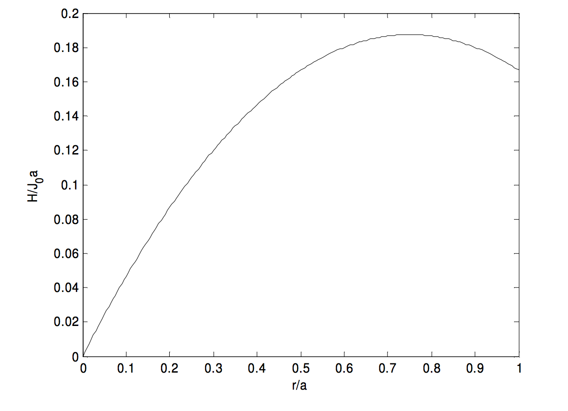
In the above example, the current density was uniform. But now we can think of lots and lots of examples in which the current density is not uniform. For example, let us imagine that we have a long straight hollow cylindrical tube of radius \(a\), perhaps a linear particle accelerator, and the current density J (amps per square metre) varies from the middle (axis) of the cylinder to its edge according to \(J(r)=J_0(1-r/a)\). The total current is, of course, \(I=2\pi \int_0^a J(r)r\,dr=\frac{1}{3}\pi a^2 J_0\) and the mean current density is \(\overline J = \frac{1}{3}J_0\).

The question, however, is: what is the magnetic field \(H\) at a distance \(r\) from the axis? Further, show that the magnetic field at the edge (circumference) of the cylinder is \(\frac{1}{6}J_0 a\), and that the field reaches a maximum value of \(\frac{3}{16}J_0 a\) at \(r=\frac{3}{4}a\).

Well, the current enclosed within a distance \(r\) from the axis is

\[\nonumber I=2\pi \int_0^r J(x)x\,dx = \pi J_0 r^2(1-\frac{2r}{3a}),\]

and this is equal to the line integral of the magnetic field around a circle of radius \(r\), which is \(2\pi rH\). Thus

\[\nonumber H=\frac{1}{2}J_0 r (1-\frac{2r}{3a}).\]

At the circumference of the cylinder, this comes to \(\frac{1}{6}J_0 a\). Calculus shows that \(H\) reaches a maximum value of \(\frac{3}{16}J_0 a\) at \(r=\frac{3}{4}a\). The graph below shows \(H/(J_0a)\) as a function of \(x/a\).

Having whetted our appetites, we can now try the same problem but with some other distributions of current density, such as

\[\textbf{1}:J(r)=J_0\left ( 1-\frac{kr}{a}\right ); \textbf{ 2}:J(r)=J_0\left ( 1-\frac{kr^2}{a^2}\right ); \textbf{ 3}:J(r)=J_0\sqrt{1-\frac{kr}{a}}; \textbf{ 4}:J(r)=J_0\sqrt{1-\frac{kr^2}{a^2}}.\nonumber\]

The mean current density is \(\overline J =\frac{2}{a^2}\int_0^a rJ(r)\,dr\), and the total current is \(\pi a^2\) times this.

The magnetic field is \(H(r)=\frac{1}{r}\int_0^r xJ(x)\,dx\).

Here are the results:

1. \[J=J_0 \left ( 1-\frac{kr}{a}\right ),\quad \overline J = J_0 \left ( 1-\frac{2k}{3}\right ),\quad H(r)=J_0\left ( \frac{r}{2}-\frac{kr^2}{3a}\right ).\]

\(H\) reaches a maximum value of \(\frac{3J_0 a}{16k}\text{ at }r=\frac{3a}{4k}\), but this maximum occurs inside the cylinder only if \(k>\frac{3}{4}\).

2. \[J=J_0\left ( 1-\frac{kr^2}{a^2}\right ),\quad \overline J = J_0(1-\frac{1}{2}k),\quad H(r)=J_0\left ( \frac{r}{2}-\frac{kr^3}{4a^2}\right ).\]

\(H\) reaches a maximum value of \(\sqrt{\frac{2}{27k}}J_0\text{ at }\frac{r}{a}=\sqrt{\frac{2}{3k}}\), but this maximum occurs inside the cylinder only if \(k>\frac{2}{3}\).

3. \[J=J_0\sqrt{1-\frac{kr}{a}},\quad \overline J = \frac{J_0}{15k^2}[8-20(1-k)^{3/2}+12(1-k)^{5/2}],\quad H(r)=\frac{2J_0 a^2}{15k^2r}\left [ 2-5 \left ( 1-\frac{kr}{a}\right )^{3/2}+3\left ( 1-\frac{kr}{a}\right )^{5/2}\right ] .\]

I have not calculated explicit formulas for the positions and values of the maxima. A maximum occurs inside the cylinder if \(k > 0.908901\).

4. \[J=J_0\sqrt{1-\frac{kr^2}{a^2}},\quad \overline J = \frac{2J_0}{3k}\left [ 1-(1-k)^{3/2} \right ],\quad H(r)=\frac{J_0 a^2}{3kr}\left [ 1-\left ( 1-\frac{kr^2}{a^2}\right )^{3/2} \right ] .\]

A maximum occurs inside the cylinder if \(k > 0.866025\).

In all of these cases, the condition that there shall be no maximum \(H\) inside the cylinder – that is, between \(r = 0\text{ and }r = a\) - is that \(\frac{J(a)}{\overline J}>\frac{1}{2}\). I believe this to be true for any axially symmetric current density distribution, though I have not proved it. I expect that a fairly simple proof could be found by someone interested.

Additional current density distributions that readers might like to investigate are

\[ J=\frac{J_0}{1+x/a}\qquad J=\frac{J_0}{1+x^2/a^2}\qquad J=\frac{J_0}{\sqrt{1+x/a}}\nonumber\]

\[J=\frac{J_0}{\sqrt{1+x^2/a^2}} \qquad J=J_0e^{-x/a} \qquad J=J_0 e^{-x^2/a^2} \nonumber\]