5.2: Antipartículas

Tanto la ecuación de Klein-Gordon como la de Dirac tienen una propiedad realmente desagradable. Dado que la relación relativista de energía es cuadrática, ambas ecuaciones tienen, para cada solución de energía positiva, una solución de energía negativa. Realmente no deseamos ver esas cosas, ¿verdad? Las energías son siempre positivas y esto es un problema real. La resolución es sorprendentemente simple, pero también muy profunda —Requiere que veamos el problema bajo una luz muy diferente.

Figura\(\PageIndex{1}\): Una imagen esquemática de los niveles en la ecuación de Dirac

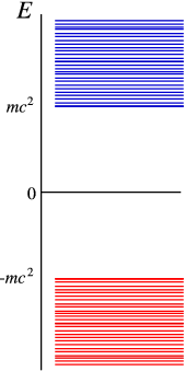
En la Figura\(\PageIndex{1}\) hemos esbozado las soluciones para la ecuación de Dirac para una partícula libre. Tiene un espectro de energía positivo a partir de\(m c^2\) (no se puede tener una partícula a menor energía), pero también un espectro de energía negativo por debajo\(-mc^2\). La interpretación de los estados de energía positiva es natural: cada estado describe una partícula que se mueve a una energía superior\(mc^2\). Como no podemos tener estados energéticos negativos, su interpretación debe ser muy diferente. La solución es simple: Asumimos que en un vacío vacío se llenan todos los estados energéticos negativos (el “mar Dirac”). Las excitaciones relativas al vacío ahora se pueden obtener agregando partículas a energías positivas o creando agujeros a energías negativas. Crear un agujero requiere energía, por lo que los estados del agujero aparecen en energías positivas. ¡Tienen carga opuesta a los estados de partículas, y así corresponderían a positrones! Esto muestra una gran similitud con el comportamiento de los semiconductores, como bien sabrás. La situación se explica en la Figura\(\PageIndex{2}\).

Figura\(\PageIndex{2}\): Imagen esquemática de los niveles ocupados y vacíos en la ecuación de Dirac. La promoción de una partícula a un nivel vacío corresponde a la creación de un par positrón-electrón, y toma una energía mayor que\(2 m c^2\).

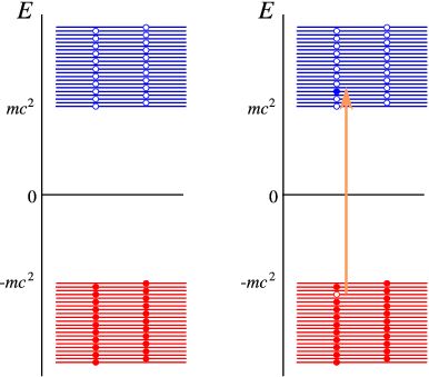
Tenga en cuenta que hemos ignorado la carga infinita del vacío (en realidad, la restamos asumiendo una carga de fondo positiva constante). La eliminación de infinidades de los cálculos es una ocurrencia frecuente en la teoría cuántica relativista (RQT). Muchas cantidades inconmensurables se vuelven infinitas, y solo nos interesa que la parte finita quede después de eliminar los infinitos. Este proceso forma parte de lo que se llama renormalización, ¡que es un procedimiento sistemático para extraer información finita de respuestas infinitas!