1.1: Variables de modelo y tipos de elementos

Flujo y Variables Transversales

El modelado de un sistema físico implica dos tipos de variables: variables de flujo que 'fluyen' a través de los componentes, y a través de variables que se miden a través de esos componentes.

Por ejemplo, en los circuitos eléctricos, el potencial (voltaje) se mide a través de los elementos, mientras que la carga eléctrica (corriente) fluye a través de los elementos del circuito.

En los sistemas de enlace mecánico, el desplazamiento y la velocidad se miden entre los elementos, mientras que la fuerza o el esfuerzo “fluye” a través de los enlaces.

En los sistemas térmicos y fluidos, el calor y la masa sirven como variables de flujo, mientras que la temperatura y la presión constituyen las variables a través.

Un elemento físico se caracteriza por la relación entre el flujo y entre variables. Los tres tipos básicos son los elementos resistivos, inductivos y capacitivos. La terminología, tomada de los circuitos eléctricos, se extiende también a otros tipos de sistemas físicos.

Mientras que el elemento resistivo disipa energía, tanto los elementos capacitivos como los inductivos almacenan energía. Por ejemplo, un condensador almacena energía eléctrica y una masa móvil almacena energía cinética. El almacenamiento de energía le da memoria al elemento que le da cuenta del comportamiento dinámico modelado por una ODE.

Dejar\(q(t)\) denotar una variable de flujo y\(x(t)\) denotar una variable transversal asociada a un elemento; entonces, el tipo de elemento se define por sus relaciones mutuas, descritas de la siguiente manera:

Definición: Elemento resistivo

Un elemento resistivo se describe mediante una relación proporcional:

\[x(t)=k\; q(t)\]

Figura\(\PageIndex{1}\): Un elemento resistivo.

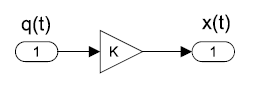
Por ejemplo, la relación voltaje y corriente a través de una resistencia se describe mediante una relación proporcional llamada ley de Ohm:\(V(t)=R\; i(t)\).

De manera similar, la relación fuerza-velocidad a través de un amortiguador mecánico lineal es proporcional:\(v(t)=\frac{1}{b} f(t)\).

Definición: Elemento capacitivo

Un elemento capacitivo se describe por la relación:

\[x(t)=k\int q(t) dt+x_{0}\]

es decir, la variable transversal varía en proporción a la cantidad acumulada de la variable de flujo. Considerando que, la variable de flujo varía proporcionalmente con la tasa de cambio de la variable transversal:

\[q\left(t\right)=\frac{1}{k}\frac{dx\left(t\right)}{dt}\]

Figura\(\PageIndex{2}\): Un elemento capacitivo.

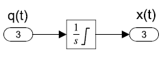
Por ejemplo, la relación de voltaje y corriente a través de un condensador se da como:\(V(t)=\frac{1}{C} \int i(t) dt+V_{0}\). Dado que la integral de corriente representa la acumulación de carga eléctrica, tenemos:\(Q=CV\). La relación inversa se describe como:\(i\left(t\right)=C\frac{dV}{dt}\).

De igual manera, la relación fuerza-velocidad que gobierna el movimiento de una masa inercial se describe como:\(v(t)=\frac{1}{m} \int f(t) dt+v_{0}\). Su inversa es la conocida segunda ley del movimiento de Newton:\(f\left(t\right)=m\frac{dv\left(t\right)}{dt}\).

Definición: Elemento inductivo

Un elemento inductivo se describe por la relación:

\[x(t)=k\frac{dq(t)}{dt}\]

es decir, la variable transversal se obtiene diferenciando la variable de flujo. Alternativamente, la variable de flujo varía en proporción a la acumulación de la variable transversal como:

\[q(t)=\frac{1}{k}\int x(t) dt+q_{0}\]

Figura\(\PageIndex{3}\): Un elemento inductivo.

Por ejemplo, la relación voltaje-corriente a través de una bobina inductiva en un circuito eléctrico se da como:\(V(t)=L\frac{di(t)}{dt}\). La relación inversa se describe como:\(i(t)=\frac{1}{L} \int V(t) dt+i_{0}\).

De manera similar, la relación fuerza-velocidad a través de un resorte lineal se da como:\(v(t)=\frac{1}{K} \frac{df(t)}{dt}\). La relación inversa se describe como:\(f\left(t\right)=K\int{v\left(t\right)dt}+f_0\).