Saltar al contenido principal
LibreTexts Español

6.5: Diagrama de manivela

  • Page ID
    86588
  • \( \newcommand{\vecs}[1]{\overset { \scriptstyle \rightharpoonup} {\mathbf{#1}} } \) \( \newcommand{\vecd}[1]{\overset{-\!-\!\rightharpoonup}{\vphantom{a}\smash {#1}}} \)\(\newcommand{\id}{\mathrm{id}}\) \( \newcommand{\Span}{\mathrm{span}}\) \( \newcommand{\kernel}{\mathrm{null}\,}\) \( \newcommand{\range}{\mathrm{range}\,}\) \( \newcommand{\RealPart}{\mathrm{Re}}\) \( \newcommand{\ImaginaryPart}{\mathrm{Im}}\) \( \newcommand{\Argument}{\mathrm{Arg}}\) \( \newcommand{\norm}[1]{\| #1 \|}\) \( \newcommand{\inner}[2]{\langle #1, #2 \rangle}\) \( \newcommand{\Span}{\mathrm{span}}\) \(\newcommand{\id}{\mathrm{id}}\) \( \newcommand{\Span}{\mathrm{span}}\) \( \newcommand{\kernel}{\mathrm{null}\,}\) \( \newcommand{\range}{\mathrm{range}\,}\) \( \newcommand{\RealPart}{\mathrm{Re}}\) \( \newcommand{\ImaginaryPart}{\mathrm{Im}}\) \( \newcommand{\Argument}{\mathrm{Arg}}\) \( \newcommand{\norm}[1]{\| #1 \|}\) \( \newcommand{\inner}[2]{\langle #1, #2 \rangle}\) \( \newcommand{\Span}{\mathrm{span}}\)\(\newcommand{\AA}{\unicode[.8,0]{x212B}}\)

    De hecho todavía tenemos algunas opciones abiertas para nosotros. Uno de los más agradables, al menos en términos de obtener alguna idea, se llama diagrama de manivela. Tenga en cuenta que esta ecuación es una ecuación compleja, la cual nos obliga a tomar la relación de dos números complejos: 1+ Γ ν e(i2βs) 1 Γ ν 2 β s y 1 Γ ν e(i2βs) 1 Γ ν 2 β s .

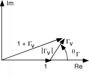
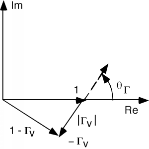
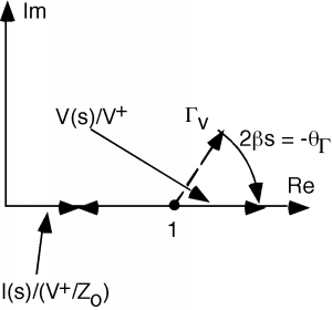
    Trazemos estas dos cantidades en el plano complejo, comenzando en s=0 s 0 (el extremo de carga de la línea). Podemos representar Γ ν Γ ν , el coeficiente de reflexión, por su magnitud y su fase, que son | Γ ν | Γ ν y φ Γ φ γ respectivamente. Para el numerador trazamos un 1, y luego agregamos el vector complejoΓΓque tiene una longitud |Γ| Γ y se sienta en ángulo φ Γ φ Γ con respecto al eje real, como se muestra en la Figura\(\PageIndex{1}\). El denominador es exactamente lo mismo, excepto que el\(\Gamma\) vector apunta en dirección opuesta como se muestra en la Figura\(\PageIndex{2}\).
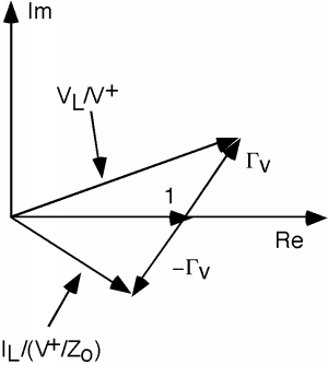
    Gráfico de primer cuadrante con componentes reales representados en el eje horizontal y componentes imaginarios representados en el eje vertical. El vector que representa 1 + gamma_V se extiende hacia arriba y hacia la derecha desde el origen. El vector que representa gamma_V, con la magnitud de Gamma_V, se extiende hacia arriba y hacia la derecha desde el valor de 1 en el eje real, en un ángulo de Theta_gamma desde el eje real. Los dos vectores se cruzan en sus cabezas.
    Figura\(\PageIndex{1}\): Plotting 1+ Γ ν 1 Γ ν
    A plot with real components represented by the x-axis and imaginary components represented by the y-axis. A vector 1 - Gamma_v extends downwards and to the right from the origin. A vector representing Gamma_v, with the magnitude of Gamma_v, extends downwards and to the left, starting at the same point as the vector for Gamma_v from Figure 1 above but heading in the opposite direction. The two vectors intersect at their heads.
    Figura\(\PageIndex{2}\): Trazado 1 Γ ν 1 Γ ν

    El vector superior es proporcional a Vs V s y el vector inferior es proporcional a Is I s, como se muestra enFigura\(\PageIndex{3}\). Por supuesto, para s=0 s 0 estamos a la carga, así que Vs=0= V L V s 0 V L y Is=0= I L I s 0 I L .

    Las dos gráficas de las Figuras 1 y 2 anteriores se representan en un solo conjunto de ejes. El vector previamente marcado con 1 + gamma_V ahora representa V_L/V+, y el vector previamente etiquetado como 1 - gamma_V ahora representa I_L/ (V+/Z_0).
    Figura\(\PageIndex{3}\): Another crank diagram showing that 1+ Γ ν = V L V + 1 Γ ν V L V + and 1 Γ ν = Z 0 I L V + 1 Γ ν Z 0 I L V +

    As we move down the line, the two "ΓΓ" vectors rotate around at a rate of -2βs -2 β as shown in Figure \(\PageIndex{4}\). As they rotate, one vector gets longer and the other gets shorter, and then the opposite occurs. In any event, to get Zs Z s we have to divide the first vector by the second. In general, this is not easy to do, but there are some places where it is not too bad. One of these is when 2βs= θ Γ 2 β s θ Γ, which is shown in Figure \(\PageIndex{5}\).
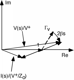
    The system of vectors from Figure 3 above is rotated a small amount clockwise so that the angle of the Gamma_v with respect to the real axis is decreased, with the rotation rate equal to 2 beta s. All contacts between heads and tails of the vectors and the vectors' points of contact with the axes that were present in Figure 3 are maintained here.

    Figura\(\PageIndex{4}\) Rotación de los fasores en el diagrama de manivela

    Continuación de la rotación del diagrama de manivela de la Figura 4 anterior, de manera que los cuatro vectores queden planos sobre el eje real. El valor de 2 beta s es igual a -Theta_gamma.
    Figura\(\PageIndex{5}\)Rotating a crank diagram to a V max V max

    At this point, the voltage vector has rotated around so that it is just lying on the real axis. Obviously its length is now 1+|Γ| 1 Γ . By the same token, the current vector is also lying on the real axis, and has a length 1|Γ| 1 Γ . Dividing one by the other, and multiplying by Z 0 Z 0 gives us Zs Z s at this point.

    Zs= Z 0 1+| Γ ν |1| Γ ν | Z s Z 0 1 Γ ν 1 Γ ν

    Where is this point, and does it have any special meaning? For this, we need to go back to our expression for Vs V s in this equation.

    Vs= V + eiβs(1+ Γ ν e-2iβs)= V + eiβs(1+| Γ ν |ei( θ Γ 2βs))= V + eiβs(1+| Γ ν |eiφs) V s V + β s 1 Γ ν -2 β s V + β s 1 Γ ν θ Γ 2 β s V + β s 1 Γ ν φ s

    where we have substituted | Γ ν |eiθ Γ ν θ for the phasor Γ ν Γ ν and then defined a new angle φs= θ Γ 2βs φ s θ Γ 2 β s .

    Now let's find the magnitude of Vs V s . To do this we need to square the real and imaginary parts, add them, and then take the square root.

    |Vs|=| V + |(1+| Γ ν |eiφs)=| V + |1+| Γ ν |cosφs2+| Γ ν |2sin2φs V s V + 1 Γ ν φ s V + 1 Γ ν φ s 2 Γ ν 2 φ s 2

    so,

    |Vs|=| V + |1+2| Γ ν |cosφs+| Γ ν |2cos2φs+| Γ ν |2sin2φs V s V + 1 2 Γ ν φ s Γ ν 2 φ s 2 Γ ν 2 φ s 2

    which, since sin2·+cos2·=1 · 2 · 2 1

    |Vs|=| V + |1+| Γ ν |2+2| Γ ν |cosφs V s V + 1 Γ ν 2 2 Γ ν φ s

    Remember, φs φ s is an angle which changes with ss. In particular, φs= θ Γ 2βs φ s θ Γ 2 β s . Thus, as we move down the line |Vs| V s will oscillate as cosφs φ s oscillates. A typical plot for Vs V s (for | Γ ν |=0.5 Γ ν 0.5 and θ Γ = 45 ° θ Γ 45 ° ) is shown below in Figure \(\PageIndex{6}\).
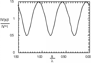
    Plot of the standing wave pattern of the magnitude of V(s) divided by the magnitude of V+, over a horizontal axis of s divided by lambda.

    Figura Patrón\(\PageIndex{6}\) de onda estacionaria


    This page titled 6.5: Diagrama de manivela is shared under a CC BY 1.0 license and was authored, remixed, and/or curated by Bill Wilson.