
6.6: Ondas estacionales/VSWR
- Page ID
- 86594

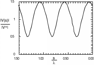
Figura\(\PageIndex{1}\): A standing wave pattern
In making this plot, we have made use of the fact that the propagation constant can also be expressed as , and so for the independent variable, instead of showing in meters or whatever, we normalize the distance away from the load to the wavelength of the excitation signal, and hence show distance in wavelengths. What we are showing here is called a standing wave. There are places along the line where the magnitude of the voltage has a maximum value. This is where and are adding up in phase with one another, and places where there is a voltage minimum, where and add up out of phase. Since , the maximum value of the standing wave pattern is times and the minimum is times . Note that anywhere on the line, the voltage is still oscillating at , and so it is not a constant, it is just that the magnitude of the oscillating signal changes as we move down the line. If we were to put an oscilloscope across the line, we would see an AC signal, oscillating at a frequency .
A number of considerable interest is the ratio of the maximum voltage amplitude to the minimum voltage amplitude, called the voltage standing wave ratio, or VSWR for short. It is easy to see that:
Note that because , .
Although Figure \(\PageIndex{1}\) looks like the standing wave pattern is more or less sinusoidal, if we increase to 0.8, we see that it most definitely is not. There is also a temptation to say that the spacing between minima (or maxima) of the standing wave pattern is , the wavelength of the signal, but a closer inspection of either Figure \(\PageIndex{1}\) or Figure \(\PageIndex{2}\) shows that in fact the spacing between features is only half a wavelength, or . Why is this? Well, goes as and , and so every time increases by , decreases by and we have come one full cycle on the way behaves.
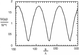
Figura Patrón\(\PageIndex{2}\): de onda estacionaria con un coeficiente de reflexión mayor
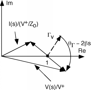
Ahora volvamos al Diagrama de manivela. En la posición que se muestra, estamos en un voltaje máximo, ysolo es igual al VSWR.
Obsérvese también que en este punto en particular, que los fasores de tensión y corriente están en fase entre sí (alineados en la misma dirección) y por lo tanto la impedancia debe ser real o resistiva.
Podemos avanzar más abajo en la línea, y ahora elfasor comienza a encogerse, y elfasor empieza a hacerse más grande Figura.
Si nos movemos aún más abajo de la línea, llegamos a un punto donde el fasor actual está ahora en un valor máximo, y el fasor de voltaje está en un valor mínimo Figura. Ahora estamos en un mínimo de voltaje, la impedancia vuelve a ser real (los fasores de voltaje y corriente están alineados entre sí, por lo que deben estar en fase) y
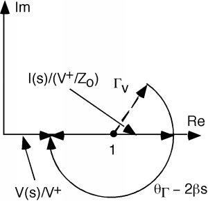
El único problema que tenemos aquí es que salvo en un voltaje mínimo o máximo, encontrandodel diagrama de manivela no es muy sencillo, ya que el voltaje y la corriente están desfasados, y dividir los dos vectores se vuelve algo tedioso.