
4.2: Respuesta de impulso de tiempo discreto
- Page ID
- 86239

\( \newcommand{\vecs}[1]{\overset { \scriptstyle \rightharpoonup} {\mathbf{#1}} } \)
\( \newcommand{\vecd}[1]{\overset{-\!-\!\rightharpoonup}{\vphantom{a}\smash {#1}}} \)
\( \newcommand{\id}{\mathrm{id}}\) \( \newcommand{\Span}{\mathrm{span}}\)
( \newcommand{\kernel}{\mathrm{null}\,}\) \( \newcommand{\range}{\mathrm{range}\,}\)
\( \newcommand{\RealPart}{\mathrm{Re}}\) \( \newcommand{\ImaginaryPart}{\mathrm{Im}}\)
\( \newcommand{\Argument}{\mathrm{Arg}}\) \( \newcommand{\norm}[1]{\| #1 \|}\)
\( \newcommand{\inner}[2]{\langle #1, #2 \rangle}\)
\( \newcommand{\Span}{\mathrm{span}}\)
\( \newcommand{\id}{\mathrm{id}}\)
\( \newcommand{\Span}{\mathrm{span}}\)
\( \newcommand{\kernel}{\mathrm{null}\,}\)
\( \newcommand{\range}{\mathrm{range}\,}\)
\( \newcommand{\RealPart}{\mathrm{Re}}\)
\( \newcommand{\ImaginaryPart}{\mathrm{Im}}\)
\( \newcommand{\Argument}{\mathrm{Arg}}\)
\( \newcommand{\norm}[1]{\| #1 \|}\)
\( \newcommand{\inner}[2]{\langle #1, #2 \rangle}\)
\( \newcommand{\Span}{\mathrm{span}}\) \( \newcommand{\AA}{\unicode[.8,0]{x212B}}\)
\( \newcommand{\vectorA}[1]{\vec{#1}} % arrow\)
\( \newcommand{\vectorAt}[1]{\vec{\text{#1}}} % arrow\)
\( \newcommand{\vectorB}[1]{\overset { \scriptstyle \rightharpoonup} {\mathbf{#1}} } \)
\( \newcommand{\vectorC}[1]{\textbf{#1}} \)
\( \newcommand{\vectorD}[1]{\overrightarrow{#1}} \)
\( \newcommand{\vectorDt}[1]{\overrightarrow{\text{#1}}} \)
\( \newcommand{\vectE}[1]{\overset{-\!-\!\rightharpoonup}{\vphantom{a}\smash{\mathbf {#1}}}} \)
\( \newcommand{\vecs}[1]{\overset { \scriptstyle \rightharpoonup} {\mathbf{#1}} } \)
\( \newcommand{\vecd}[1]{\overset{-\!-\!\rightharpoonup}{\vphantom{a}\smash {#1}}} \)
\(\newcommand{\avec}{\mathbf a}\) \(\newcommand{\bvec}{\mathbf b}\) \(\newcommand{\cvec}{\mathbf c}\) \(\newcommand{\dvec}{\mathbf d}\) \(\newcommand{\dtil}{\widetilde{\mathbf d}}\) \(\newcommand{\evec}{\mathbf e}\) \(\newcommand{\fvec}{\mathbf f}\) \(\newcommand{\nvec}{\mathbf n}\) \(\newcommand{\pvec}{\mathbf p}\) \(\newcommand{\qvec}{\mathbf q}\) \(\newcommand{\svec}{\mathbf s}\) \(\newcommand{\tvec}{\mathbf t}\) \(\newcommand{\uvec}{\mathbf u}\) \(\newcommand{\vvec}{\mathbf v}\) \(\newcommand{\wvec}{\mathbf w}\) \(\newcommand{\xvec}{\mathbf x}\) \(\newcommand{\yvec}{\mathbf y}\) \(\newcommand{\zvec}{\mathbf z}\) \(\newcommand{\rvec}{\mathbf r}\) \(\newcommand{\mvec}{\mathbf m}\) \(\newcommand{\zerovec}{\mathbf 0}\) \(\newcommand{\onevec}{\mathbf 1}\) \(\newcommand{\real}{\mathbb R}\) \(\newcommand{\twovec}[2]{\left[\begin{array}{r}#1 \\ #2 \end{array}\right]}\) \(\newcommand{\ctwovec}[2]{\left[\begin{array}{c}#1 \\ #2 \end{array}\right]}\) \(\newcommand{\threevec}[3]{\left[\begin{array}{r}#1 \\ #2 \\ #3 \end{array}\right]}\) \(\newcommand{\cthreevec}[3]{\left[\begin{array}{c}#1 \\ #2 \\ #3 \end{array}\right]}\) \(\newcommand{\fourvec}[4]{\left[\begin{array}{r}#1 \\ #2 \\ #3 \\ #4 \end{array}\right]}\) \(\newcommand{\cfourvec}[4]{\left[\begin{array}{c}#1 \\ #2 \\ #3 \\ #4 \end{array}\right]}\) \(\newcommand{\fivevec}[5]{\left[\begin{array}{r}#1 \\ #2 \\ #3 \\ #4 \\ #5 \\ \end{array}\right]}\) \(\newcommand{\cfivevec}[5]{\left[\begin{array}{c}#1 \\ #2 \\ #3 \\ #4 \\ #5 \\ \end{array}\right]}\) \(\newcommand{\mattwo}[4]{\left[\begin{array}{rr}#1 \amp #2 \\ #3 \amp #4 \\ \end{array}\right]}\) \(\newcommand{\laspan}[1]{\text{Span}\{#1\}}\) \(\newcommand{\bcal}{\cal B}\) \(\newcommand{\ccal}{\cal C}\) \(\newcommand{\scal}{\cal S}\) \(\newcommand{\wcal}{\cal W}\) \(\newcommand{\ecal}{\cal E}\) \(\newcommand{\coords}[2]{\left\{#1\right\}_{#2}}\) \(\newcommand{\gray}[1]{\color{gray}{#1}}\) \(\newcommand{\lgray}[1]{\color{lightgray}{#1}}\) \(\newcommand{\rank}{\operatorname{rank}}\) \(\newcommand{\row}{\text{Row}}\) \(\newcommand{\col}{\text{Col}}\) \(\renewcommand{\row}{\text{Row}}\) \(\newcommand{\nul}{\text{Nul}}\) \(\newcommand{\var}{\text{Var}}\) \(\newcommand{\corr}{\text{corr}}\) \(\newcommand{\len}[1]{\left|#1\right|}\) \(\newcommand{\bbar}{\overline{\bvec}}\) \(\newcommand{\bhat}{\widehat{\bvec}}\) \(\newcommand{\bperp}{\bvec^\perp}\) \(\newcommand{\xhat}{\widehat{\xvec}}\) \(\newcommand{\vhat}{\widehat{\vvec}}\) \(\newcommand{\uhat}{\widehat{\uvec}}\) \(\newcommand{\what}{\widehat{\wvec}}\) \(\newcommand{\Sighat}{\widehat{\Sigma}}\) \(\newcommand{\lt}{<}\) \(\newcommand{\gt}{>}\) \(\newcommand{\amp}{&}\) \(\definecolor{fillinmathshade}{gray}{0.9}\)Introducción
La salida de un sistema LTI de tiempo discreto está completamente determinada por la entrada y la respuesta del sistema a un impulso unitario.
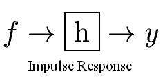
![Un sistema de tiempo discreto H toma la entrada x [n] y produce la salida y [n].](https://eng.libretexts.org/@api/deki/files/20274/hsystem.PNG)
La salida para una entrada de impulso de unidad se llama respuesta de impulso.
![Una entrada de impulso delta [n] que pasa por un sistema de tiempo discreto H, produciendo la respuesta de impulso del sistema, h [n].](https://eng.libretexts.org/@api/deki/files/20273/impulse.PNG)
Figura\(\PageIndex{2}\)
![delta [n] 'choca' el sistema repentinamente.](https://eng.libretexts.org/@api/deki/files/20271/g1.png) a)
a)![h [n] es la respuesta al choque.](https://eng.libretexts.org/@api/deki/files/20275/g2.png) b)
b)
Figura\(\PageIndex{3}\)
Impulsos de ejemplo
Dado que estamos considerando señales de tiempo discretas y sistemas, un impulso ideal es fácil de simular en una computadora o algún otro dispositivo digital. Es simplemente una señal que es 1 en el punto\(n\) = 0, y 0 en todas partes.
Sistemas LTI y Respuestas al Impulso
Encontrar salidas del sistema
Por la propiedad de tamizado de los impulsos, cualquier señal puede descomponerse en términos de una suma infinita de impulsos desplazados y escalados.
\ [\ begin {align}
x [n] &=\ suma_ {k=-\ infty} ^ {\ infty} x [k]\ delta_ {k} [n]\ nonumber\\
&=\ sum_ {k=-\ infty} ^ {\ infty} x [k]\ delta [n-k]
\ end {align}\ nonumber\]
La función\(\delta_{k}[\mathrm{n}]=\delta[\mathrm{n}-\mathrm{k}]\) alcanza su punto máximo donde\(n=k\).
![La función δ [n-k]. Simplemente es 1 en el punto n y 0 en todas partes. El punto n está marcado en la gráfica.](https://eng.libretexts.org/@api/deki/files/20272/s1.png) a)
a)![La función x [k]. Tiene una forma extraña. El punto n está marcado en la gráfica.](https://eng.libretexts.org/@api/deki/files/20281/s2.png) b)
b)
Figura\(\PageIndex{4}\)
Como conocemos la respuesta del sistema a un impulso y cualquier señal puede descomponerse en impulsos, todo lo que necesitamos hacer para encontrar la respuesta del sistema a cualquier señal es descomponer la señal en impulsos, calcular la salida del sistema para cada impulso y sumar las salidas nuevamente juntas. Este es el proceso conocido como Convolución. Como estamos en Tiempo Discreto, esta es la Suma de Convolución de Tiempo Discreto.
Encontrar respuestas de impulso
Teoría:
- Resuelve la Ecuación de Diferencia del sistema para y [n] con f [n] = δ [n]
- Utilice la transformación Z
Práctica:
- Aplique una señal de entrada de impulso al sistema y registre la salida
- Usar métodos de Fourier
Supondremos que\(h[n]\) se da por ahora. El objetivo ahora es calcular la salida\(y[n]\) dada la respuesta de impulso\(h[n]\) y la entrada\(x[n]\).
Figura\(\PageIndex{5}\)
Resumen de respuesta al impulso
Cuando un sistema es “conmocionado” por una función delta, produce una salida conocida como su respuesta de impulso. Para un sistema LTI, la respuesta de impulso determina completamente la salida del sistema dada cualquier entrada arbitraria. La salida se puede encontrar usando convolución de tiempo discreta.