7.3: Serie Discreta Común de Fourier

Introducción

Una vez que se ha obtenido una comprensión sólida de los fundamentos del análisis de series de Fourier y la Derivación General de los Coeficientes de Fourier, es útil tener una comprensión de las señales comunes utilizadas en la Aproximación de Señales de la Serie de Fourier.

Derivando los Coeficientes

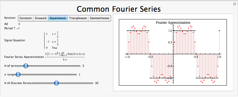
Considera una onda cuadrada\(f(x)\) de longitud 1. En el rango [0,1), esto se puede escribir como

\ [x (t) =\ left\ {\ begin {array} {rl}
1 & t\ leq\ frac {1} {2}\\
-1 & t>\ frac {1} {2}
\ end {array}\ right. \ nonumber\]

Aproximación en serie de Fourier de una onda cuadrada

Figura\(\PageIndex{1}\): Aproximación de la serie de Fourier a\(sq(t)\). El número de términos en la suma de Fourier se indica en cada gráfica, y la onda cuadrada se muestra como una línea discontinua en dos periodos.

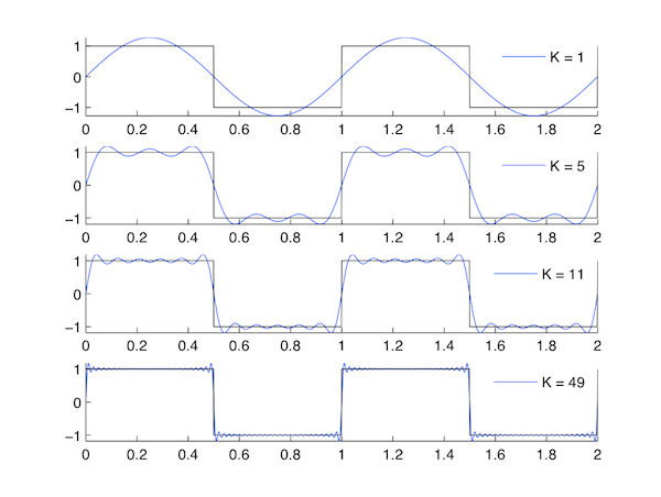
Real Even Signals Dado que la onda cuadrada es una señal real y uniforme,

• \(f(t)=f(−t)\)INCLUSO
• \(f(t)=f^*(t)\)REAL

por lo tanto,

• \(c_n=c_{−n}\)INCLUSO
• \(c_n=c_n^*\)REAL

Derivación de los Coeficientes para otras señales

La onda cuadrada es el ejemplo estándar, pero otras señales importantes también son útiles para analizar, y estas se incluyen aquí.

Forma de onda constante

Esta señal es relativamente autoexplicativa: se saca la porción variable en el tiempo del Coeficiente de Fourier, y nos quedamos simplemente con una función constante en todo el tiempo.

\[x(t)=1 \nonumber \]

Aproximación en serie de Fourier de una onda constante

Figura\(\PageIndex{2}\)

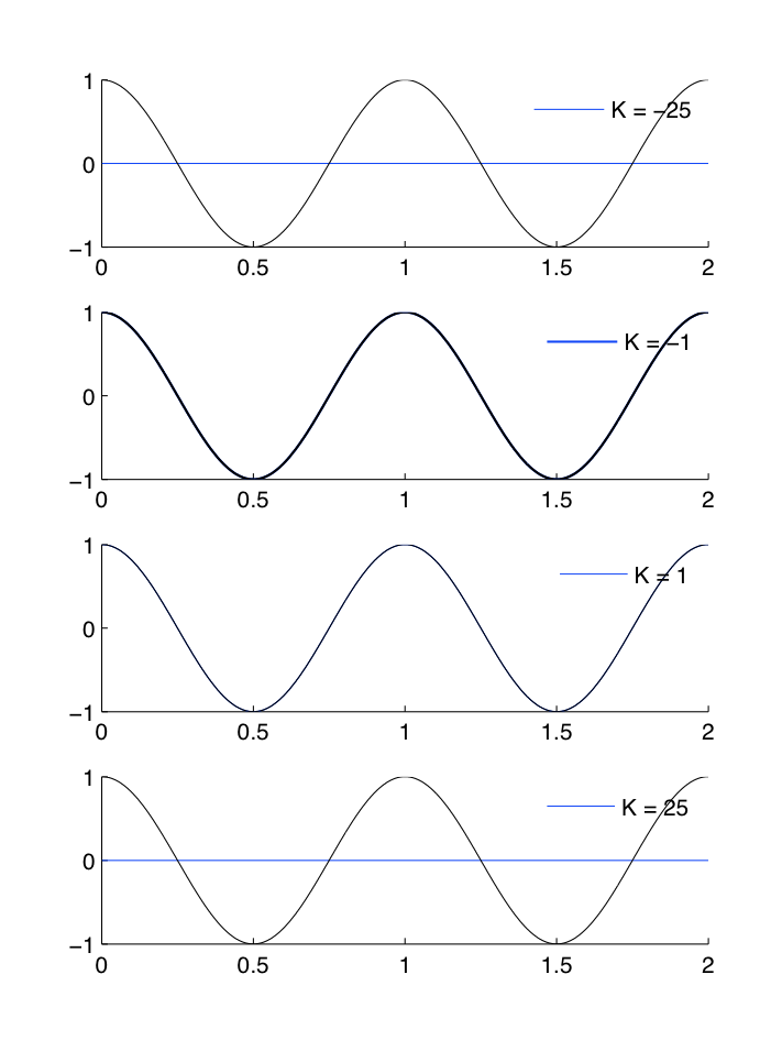
Forma de onda sinusoidal

Con esta señal, solo se elige una frecuencia específica de Coeficiente variable en el tiempo (dado que la ecuación de la Serie de Fourier incluye una onda sinusoidal, esto es intuitivo), y todas las demás se filtran, y este único coeficiente variable en el tiempo coincidirá exactamente con la señal deseada.

\[x(t)=\cos (2 \pi t) \nonumber \]

Aproximación en serie de Fourier de una onda sinusoidal

Figura\(\PageIndex{3}\)

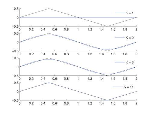
Forma de onda triangular

\ [x (t) =\ left\ {\ begin {array} {rl}
t & t\ leq 1/2\\
1-t & t>1/2
\ end {array}\ right. \ nonumber\]

Esta es una forma más compleja de aproximación de señal a la onda cuadrada. Debido a las Propiedades de Simetría de la Serie de Fourier, la onda triangular es una señal real e impar, a diferencia de la señal de onda cuadrada real y par. Esto significa que

• \(f(t)=−f(−t)\)ODD
• \(f(t)=f^*(t)\)REAL

por lo tanto,

• \(c_n=−c_{−n}\)
• \(c_n=−c_n^*\)Imaginario

Aproximación de la serie de Fourier de una onda triangular

Figura\(\PageIndex{4}\)

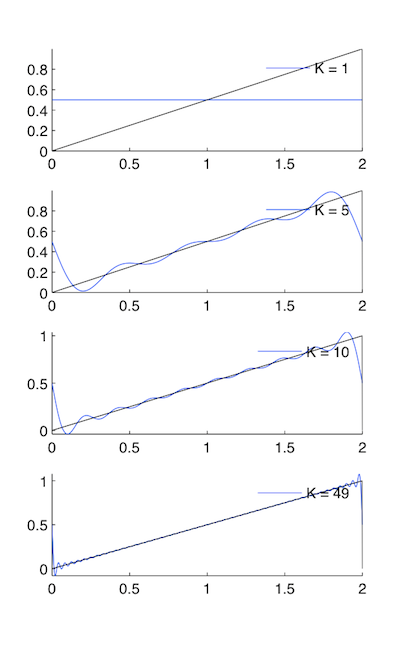
Forma de onda de diente de

\[x(t) = t/2 \nonumber \]

Debido a las propiedades de simetría de la serie de Fourier, la onda en diente de sierra se puede definir como una señal real e impar, a diferencia de la señal de onda cuadrada real y par. Esto tiene implicaciones importantes para los Coeficientes de Fourier.

Aproximación en serie de Fourier de una onda en diente de sierra

Figura\(\PageIndex{5}\)

Aproximación de señal DFT

Figura\(\PageIndex{6}\): Interactuar (cuando esté en línea) con un CDF de Mathematica demostrando la serie común de Fourier Discreta. Para descargar, haga clic derecho y guárdalos como .cdf.

Conclusión

En resumen, existe una gran variedad entre las Transformadas de Fourier comunes. Aquí se proporciona una tabla resumida con la información esencial.

Tabla\(\PageIndex{1}\): Transformadas de Fourier discretas comunes

Descripción	Señal de dominio de tiempo para\(n \in \mathbb{Z}[0, N-1]\)	Señal de dominio de frecuencia\(k \in \mathbb{Z}[0, N-1]\)
Función Constante	1	\(\delta(k)\)
Impulso de Unidad	\(\delta(n)\)	\(\frac{1}{N}\)
Exponencial Complejo	\(e^{j 2 \pi m n / N}\)	\(\delta\left((k-m)_{N}\right)\)
Forma de onda sinusoidal	\(\cos (j 2 \pi m n / N)\)	\(\frac{1}{2}\left(\delta\left((k-m)_{N}\right)+\delta\left((k+m)_{N}\right)\right)\)
Forma de onda de caja\((M < N/2)\)	\(\delta(n)+\sum_{m=1}^{M} \delta\left((n-m)_{N}\right)+\delta\left((n+m)_{N}\right)\)	\(\frac{\sin ((2 M+1) k \pi / N)}{N \sin (k \pi / N)}\)
Forma de onda Dsinc\((M<N/2)\)	\(\frac{\sin ((2 M+1) n \pi / N)}{\sin (n \pi / N)}\)	\(\delta(k)+\sum_{m=1}^{M} \delta\left((k-m)_{N}\right)+\delta((k+m)_N)\)