6.2: Forma polar
- Page ID
- 114474
\( \newcommand{\vecs}[1]{\overset { \scriptstyle \rightharpoonup} {\mathbf{#1}} } \)
\( \newcommand{\vecd}[1]{\overset{-\!-\!\rightharpoonup}{\vphantom{a}\smash {#1}}} \)
\( \newcommand{\id}{\mathrm{id}}\) \( \newcommand{\Span}{\mathrm{span}}\)
( \newcommand{\kernel}{\mathrm{null}\,}\) \( \newcommand{\range}{\mathrm{range}\,}\)
\( \newcommand{\RealPart}{\mathrm{Re}}\) \( \newcommand{\ImaginaryPart}{\mathrm{Im}}\)
\( \newcommand{\Argument}{\mathrm{Arg}}\) \( \newcommand{\norm}[1]{\| #1 \|}\)
\( \newcommand{\inner}[2]{\langle #1, #2 \rangle}\)
\( \newcommand{\Span}{\mathrm{span}}\)
\( \newcommand{\id}{\mathrm{id}}\)
\( \newcommand{\Span}{\mathrm{span}}\)
\( \newcommand{\kernel}{\mathrm{null}\,}\)
\( \newcommand{\range}{\mathrm{range}\,}\)
\( \newcommand{\RealPart}{\mathrm{Re}}\)
\( \newcommand{\ImaginaryPart}{\mathrm{Im}}\)
\( \newcommand{\Argument}{\mathrm{Arg}}\)
\( \newcommand{\norm}[1]{\| #1 \|}\)
\( \newcommand{\inner}[2]{\langle #1, #2 \rangle}\)
\( \newcommand{\Span}{\mathrm{span}}\) \( \newcommand{\AA}{\unicode[.8,0]{x212B}}\)
\( \newcommand{\vectorA}[1]{\vec{#1}} % arrow\)
\( \newcommand{\vectorAt}[1]{\vec{\text{#1}}} % arrow\)
\( \newcommand{\vectorB}[1]{\overset { \scriptstyle \rightharpoonup} {\mathbf{#1}} } \)
\( \newcommand{\vectorC}[1]{\textbf{#1}} \)
\( \newcommand{\vectorD}[1]{\overrightarrow{#1}} \)
\( \newcommand{\vectorDt}[1]{\overrightarrow{\text{#1}}} \)
\( \newcommand{\vectE}[1]{\overset{-\!-\!\rightharpoonup}{\vphantom{a}\smash{\mathbf {#1}}}} \)
\( \newcommand{\vecs}[1]{\overset { \scriptstyle \rightharpoonup} {\mathbf{#1}} } \)
\( \newcommand{\vecd}[1]{\overset{-\!-\!\rightharpoonup}{\vphantom{a}\smash {#1}}} \)
\(\newcommand{\avec}{\mathbf a}\) \(\newcommand{\bvec}{\mathbf b}\) \(\newcommand{\cvec}{\mathbf c}\) \(\newcommand{\dvec}{\mathbf d}\) \(\newcommand{\dtil}{\widetilde{\mathbf d}}\) \(\newcommand{\evec}{\mathbf e}\) \(\newcommand{\fvec}{\mathbf f}\) \(\newcommand{\nvec}{\mathbf n}\) \(\newcommand{\pvec}{\mathbf p}\) \(\newcommand{\qvec}{\mathbf q}\) \(\newcommand{\svec}{\mathbf s}\) \(\newcommand{\tvec}{\mathbf t}\) \(\newcommand{\uvec}{\mathbf u}\) \(\newcommand{\vvec}{\mathbf v}\) \(\newcommand{\wvec}{\mathbf w}\) \(\newcommand{\xvec}{\mathbf x}\) \(\newcommand{\yvec}{\mathbf y}\) \(\newcommand{\zvec}{\mathbf z}\) \(\newcommand{\rvec}{\mathbf r}\) \(\newcommand{\mvec}{\mathbf m}\) \(\newcommand{\zerovec}{\mathbf 0}\) \(\newcommand{\onevec}{\mathbf 1}\) \(\newcommand{\real}{\mathbb R}\) \(\newcommand{\twovec}[2]{\left[\begin{array}{r}#1 \\ #2 \end{array}\right]}\) \(\newcommand{\ctwovec}[2]{\left[\begin{array}{c}#1 \\ #2 \end{array}\right]}\) \(\newcommand{\threevec}[3]{\left[\begin{array}{r}#1 \\ #2 \\ #3 \end{array}\right]}\) \(\newcommand{\cthreevec}[3]{\left[\begin{array}{c}#1 \\ #2 \\ #3 \end{array}\right]}\) \(\newcommand{\fourvec}[4]{\left[\begin{array}{r}#1 \\ #2 \\ #3 \\ #4 \end{array}\right]}\) \(\newcommand{\cfourvec}[4]{\left[\begin{array}{c}#1 \\ #2 \\ #3 \\ #4 \end{array}\right]}\) \(\newcommand{\fivevec}[5]{\left[\begin{array}{r}#1 \\ #2 \\ #3 \\ #4 \\ #5 \\ \end{array}\right]}\) \(\newcommand{\cfivevec}[5]{\left[\begin{array}{c}#1 \\ #2 \\ #3 \\ #4 \\ #5 \\ \end{array}\right]}\) \(\newcommand{\mattwo}[4]{\left[\begin{array}{rr}#1 \amp #2 \\ #3 \amp #4 \\ \end{array}\right]}\) \(\newcommand{\laspan}[1]{\text{Span}\{#1\}}\) \(\newcommand{\bcal}{\cal B}\) \(\newcommand{\ccal}{\cal C}\) \(\newcommand{\scal}{\cal S}\) \(\newcommand{\wcal}{\cal W}\) \(\newcommand{\ecal}{\cal E}\) \(\newcommand{\coords}[2]{\left\{#1\right\}_{#2}}\) \(\newcommand{\gray}[1]{\color{gray}{#1}}\) \(\newcommand{\lgray}[1]{\color{lightgray}{#1}}\) \(\newcommand{\rank}{\operatorname{rank}}\) \(\newcommand{\row}{\text{Row}}\) \(\newcommand{\col}{\text{Col}}\) \(\renewcommand{\row}{\text{Row}}\) \(\newcommand{\nul}{\text{Nul}}\) \(\newcommand{\var}{\text{Var}}\) \(\newcommand{\corr}{\text{corr}}\) \(\newcommand{\len}[1]{\left|#1\right|}\) \(\newcommand{\bbar}{\overline{\bvec}}\) \(\newcommand{\bhat}{\widehat{\bvec}}\) \(\newcommand{\bperp}{\bvec^\perp}\) \(\newcommand{\xhat}{\widehat{\xvec}}\) \(\newcommand{\vhat}{\widehat{\vvec}}\) \(\newcommand{\uhat}{\widehat{\uvec}}\) \(\newcommand{\what}{\widehat{\wvec}}\) \(\newcommand{\Sighat}{\widehat{\Sigma}}\) \(\newcommand{\lt}{<}\) \(\newcommand{\gt}{>}\) \(\newcommand{\amp}{&}\) \(\definecolor{fillinmathshade}{gray}{0.9}\)- Convierta un número complejo de forma estándar a forma polar, y de forma polar a forma estándar.
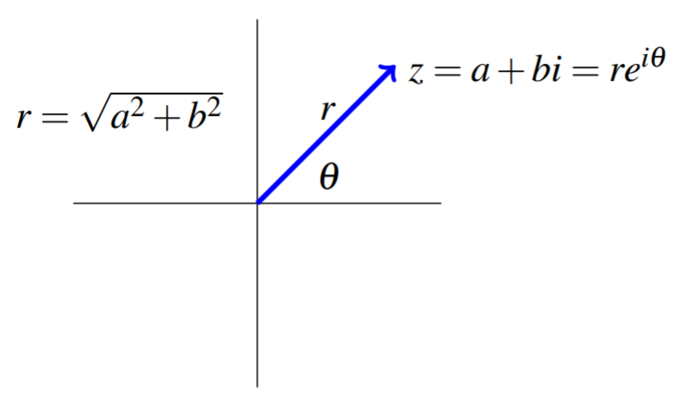
En la sección anterior, identificamos un número complejo\(z=a+bi\) con un punto\(\left( a, b\right)\) en el plano de coordenadas. Hay otra forma en la que podemos expresar el mismo número, llamada la forma polar. La forma polar es el foco de esta sección. Se va a resultar muy útil si no crucial para ciertos cálculos como pronto veremos.
Supongamos que\(z=a+bi\) es un número complejo, y vamos\(r=\sqrt{a^{2}+b^{2}} = |z|\). Recordemos que\(r\) es el módulo de\(z\). Tenga en cuenta primero que\[\left( \frac{a}{r} \right) ^{2}+\left( \frac{b}{r}\right) ^{2}= \frac{a^2+b^2}{r^2}=1\nonumber\] y así\(\left( \frac{a}{r},\frac{b}{r}\right)\) es un punto en el círculo unitario. Por lo tanto, existe un ángulo\(\theta\) (en radianes) tal que\[\cos \theta =\frac{a}{r},\ \sin \theta =\frac{b}{r}\nonumber\] en otras palabras\(\theta\) es un ángulo tal que\(a = r\cos \theta\) y\(b=r \sin \theta\), es decir\(\theta = \cos^{-1}(a/r)\) y\(\theta = \sin^{-1}(b/r)\). Llamamos a este ángulo\(\theta\) el argumento de\(z\).
A menudo hablamos del argumento principal de\(z\). Este es el ángulo único\(\theta \in (-\pi, \pi]\) tal que\[\cos \theta =\frac{a}{r},\ \sin \theta =\frac{b}{r}\nonumber\]
La forma polar del número complejo\(z=a+bi = r \left( \cos \theta +i\sin \theta \right)\) se escribe por conveniencia como:\[z = r e^{i \theta}\nonumber\] dónde\(\theta\) está el argumento de\(z\).
Dejar\(z = a + bi\) ser un número complejo. Entonces la forma polar de\(z\) se escribe como\[z = re^{i\theta}\nonumber\] dónde\(r = \sqrt{a^2 + b^2}\) y\(\theta\) es el argumento de\(z\).
Cuando se le da\(z = re^{i\theta}\), la identidad\(e^{i\theta} = \cos\theta + i \sin\theta\) se convertirá de\(z\) nuevo a forma estándar. Aquí pensamos en\(e^{i \theta}\) como un atajo para\(\cos \theta +i\sin \theta\). Esto es todo lo que necesitaremos en este curso, pero en realidad se\(e^{i \theta}\) puede considerar como el complejo equivalente de la función exponencial donde esto resulta ser una verdadera igualdad.

Así podemos convertir cualquier número complejo en la forma estándar (cartesiana)\(z = a+bi\) en su forma polar. Considera el siguiente ejemplo.
Dejar\(z = 2 + 2i\) ser un número complejo. Escribir\(z\) en la forma polar\[z = re^{i \theta}\nonumber\]
Solución
Primero, encuentra\(r\). Por la discusión anterior,\(r=\sqrt{ a^{2}+b^{2}} = |z|\). Por lo tanto,\[r = \sqrt{2^{2} + 2^{2}} = \sqrt{8} =2\sqrt{2}\nonumber \]
Ahora, para encontrar\(\theta\), trazamos el punto\(\left( 2, 2 \right)\) y encontramos el ángulo desde el\(x\) eje positivo hasta la línea entre este punto y el origen. En este caso,\(\theta = 45^{\circ} = \frac{\pi}{4}\). Es decir encontramos el ángulo único\(\theta\) tal que\(\theta = \cos^{-1}(1/\sqrt{2})\) y\(\theta = \sin^{-1}(1/\sqrt{2})\).
Tenga en cuenta que en forma polar, siempre expresamos ángulos en radianes, no grados.
Por lo tanto, podemos escribir\(z\) como\[z = 2\sqrt{2} e^{i\frac{\pi}{4}}\nonumber\]
Observe que las formas estándar y polares son completamente equivalentes. Eso no solo podemos transformar un número complejo de forma estándar a su forma polar, también podemos tomar un número complejo en forma polar y convertirlo de nuevo a forma estándar.
Vamos\(z = 2 e^{ 2\pi i/3}\). Escribir\(z\) en la forma estándar\[z = a+bi\nonumber \]
Solución
Dejar\(z = 2 e^{2\pi i/3}\) ser la forma polar de un número complejo. Recordemos eso\(e^{i\theta} = \cos \theta + i \sin \theta\). Por lo tanto, usando valores estándar de\(\sin\) y\(\cos\) obtenemos:\[\begin{aligned} z = 2 e^{i 2\pi/3} &= 2 (\cos (2\pi/3)+i\sin (2\pi/3))\\ &= 2 \left ( -\frac{1}{2} + i \frac{\sqrt{3}}{2} \right) \\ &=-1 + \sqrt{3}i \end{aligned}\] que es la forma estándar de este número complejo.
Siempre puedes verificar tu respuesta convirtiéndola de nuevo a forma polar y asegurándote de llegar a la respuesta original.