7.1: El Método Euler

Ver tutorial en YouTube

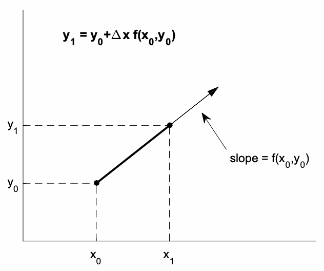
Aunque no siempre es posible encontrar una solución analítica de la Ecuación\ ref {7.1} para\(y=\)\(y(x)\), siempre es posible determinar una solución numérica única dado un valor inicial\(y\left(x_{0}\right)=y_{0}\), y siempre\(f(x, y)\) es un buen comportamiento función. La ecuación diferencial Ecuación\ ref {7.1} nos da la pendiente\(f\left(x_{0}, y_{0}\right)\) de la línea tangente a la curva de solución\(y=y(x)\) en el punto\(\left(x_{0}, y_{0}\right)\). Con un tamaño de paso pequeño\(\Delta x=x_{1}-x_{0}\), la condición inicial\(\left(x_{0}, y_{0}\right)\) puede marchar hacia adelante a\(\left(x_{1}, y_{1}\right)\) lo largo de la línea tangente usando el método de Euler (ver Fig. 7.1)

\[y_{1}=y_{0}+\Delta x f\left(x_{0}, y_{0}\right) \nonumber \]

Esta solución se convierte\(\left(x_{1}, y_{1}\right)\) entonces en la nueva condición inicial y se marcha hacia adelante a\(\left(x_{2}, y_{2}\right)\) lo largo de una línea tangente recién determinada con pendiente dada por\(f\left(x_{1}, y_{1}\right)\). Por lo suficientemente pequeña\(\Delta x\), la solución numérica converge a la solución exacta.

\[y_{1}=y_{0}+\Delta x f\left(x_{0}, y_{0}\right) \nonumber \]

Figura 7.1: La ecuación diferencial\(d y / d x=f(x, y), y\left(x_{0}\right)=y_{0}\), se integra al\(x=x_{1}\) uso del método de Euler\(y_{1}=y_{0}+\Delta x f\left(x_{0}, y_{0}\right)\), con\(\Delta x=x_{1}-x_{0}\).