3.1: El Método Euler

Ver tutorial en YouTube

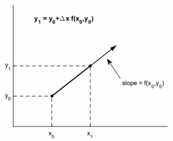
Aunque no siempre es posible encontrar una solución analítica de (3.1) para\(y = y(x)\), siempre es posible determinar una solución numérica única dado un valor inicial\(y(x_0) = y_0\), y siempre\(f(x, y)\) es una función de buen comportamiento. La ecuación diferencial (3.1) nos da la pendiente\(f(x_0, y_0)\) de la línea tangente a la curva de solución\(y = y(x)\) en el punto\((x_0, y_0)\). Con un tamaño de paso pequeño\(∆x = x_1 − x_0\), la condición inicial\((x_0, y_0)\) puede marchar hacia adelante a\((x_1, y_1)\) lo largo de la línea tangente usando el método de Euler (ver Fig. \(\PageIndex{1}\))\[y_1=y_0+\Delta xf(x_0, y_0).\nonumber\]

Esta solución se convierte\((x_1, y_1)\) entonces en la nueva condición inicial y se marcha hacia adelante a\((x_2, y_2)\) lo largo de una línea tangente recién determinada con pendiente dada por\(f(x_1, y_1)\). Por lo suficientemente pequeña\(∆x\), la solución numérica converge a la solución exacta.

Figura\(\PageIndex{1}\): La ecuación diferencial\(dy/dx = f(x, y),\)\(y(x_0) = y_0,\) se integra al\(x = x_1\) uso del método de Euler\(y_1 = y_0 + ∆x f(x_0, y_0)\), con\(∆x = x_1 − x_0\).