8.5: Ecuaciones de coeficiente constante con funciones de forzamiento continuo por tramos
- Page ID
- 114880

Ahora consideraremos problemas de valor inicial de la forma
\[\label{eq:8.5.1} ay''+by'+cy=f(t), \quad y(0)=k_0,\quad y'(0)=k_1,\]
donde\(a\),\(b\), y\(c\) son constantes (\(a\ne0\)) y\(f\) es continuo por tramos en\([0,\infty)\). Problemas de este tipo ocurren en situaciones en las que la entrada a un sistema físico sufre cambios instantáneos, como cuando se enciende o apaga un interruptor o las fuerzas que actúan sobre el sistema cambian abruptamente.
Se puede demostrar (Ejercicios 8.5.23 y 8.5.24) que la ecuación diferencial en la Ecuación\ ref {eq:8.5.1} no tiene soluciones en un intervalo abierto que contenga una discontinuidad de salto de\(f\). Por lo tanto debemos definir a qué nos referimos con una solución de la Ecuación\ ref {eq:8.5.1} on\([0,\infty)\) en el caso donde\(f\) tiene discontinuidades de salto. El siguiente teorema motiva nuestra definición. Omitimos la prueba.
Supongamos\(a,b\), y\(c\) son constantes\((a\ne0),\) y\(f\) es continuo por tramos\([0,\infty).\) con discontinuidades de salto en\(t_1,\)...,\(t_n,\) donde
\[0<t_1<\cdots<t_n. \nonumber\]
Dejemos\(k_0\) y\(k_1\) sean números reales arbitrarios. Luego hay una función única\(y\) definida\([0,\infty)\) con estas propiedades:
- \(y(0)=k_0\)y\(y'(0)=k_1\).
- \(y\)y\(y'\) son continuos en\([0,\infty)\).
- \(y''\)se define en cada subintervalo abierto de\([0,\infty)\) que no contenga ninguno de los puntos\(t_1,\)...\(t_n\), y\[ay''+by'+cy=f(t) \nonumber\] en cada uno de esos subintervalos.
- \(y''\)tiene límites desde la derecha y la izquierda en\(t_1,\)...\(,\)\(t_n\).
Definimos la función\(y\) del Teorema 8.5.1 para que sea la solución del problema del valor inicial Ecuación\ ref {eq:8.5.1}.
Comenzamos por considerar problemas de valor inicial de la forma
\[\label{eq:8.5.2} ay''+by'+cy=\left\{\begin{array}{cl} f_0(t),&0\le t<t_1,\\[4pt]f_1(t),&t\ge t_1, \end{array}\right.\quad y(0)=k_0,\quad y'(0)=k_1,\]
donde la función de forzamiento tiene una sola discontinuidad de salto en\(t_1\).
Podemos resolver la Ecuación\ ref {eq:8.5.2} por los siguientes pasos:
- Paso 1. Encuentra la solución\(y_0\) del problema de valor inicial\[ay''+by'+cy=f_0(t), \quad y(0)=k_0,\quad y'(0)=k_1. \nonumber \]
- Paso 2. Cómputos\(c_0=y_0(t_1)\) y\(c_1=y_0'(t_1)\).
- Paso 3. Encuentra la solución\(y_1\) del problema de valor inicial\[ay''+by'+cy=f_1(t), \quad y(t_1)=c_0,\quad y'(t_1)=c_1.\nonumber\]
- Paso 4. Obtener la solución\(y\) de la Ecuación\ ref {eq:8.5.2} como\[y=\left\{\begin{array}{cl} y_0(t),&0\le t<t_1\\[4pt]y_1(t),&t\ge t_1. \end{array}\right.\nonumber\]
Se muestra en el Ejercicio 8.5.23 que\(y'\) existe y es continuo en\(t_1\). El siguiente ejemplo ilustra este procedimiento.
Resolver el problema de valor inicial
\[\label{eq:8.5.3} y''+y=f(t), \quad y(0)=2,\; y'(0)=-1,\]
donde
\[f(t)=\left\{\begin{array}{rl} 1,&0\le t< \pi\over2,\\[4pt] -1,&t\ge {\pi\over2}. \end{array}\right. \nonumber\]
Solución
El problema de valor inicial en el paso 1 es
\[y''+y=1, \quad y(0)=2,\quad y'(0)=-1. \nonumber\]
Te dejamos a ti verificar que su solución es
\[y_0=1+\cos t-\sin t. \nonumber\]
Haciendo Paso 2 rinde\(y_0(\pi/2)=0\) y\(y_0'(\pi/2)=-1\), entonces el segundo problema de valor inicial es
\[y''+y=-1, \quad y\left({\pi\over2}\right)=0,\; y'\left({\pi\over 2}\right)=-1. \nonumber\]
Te dejamos verificar que la solución de este problema es
\[y_1=-1+\cos t+\sin t. \nonumber\]
De ahí que la solución de la Ecuación\ ref {eq:8.5.3} es
\[\label{eq:8.5.4} y=\left\{\begin{array}{rl} 1+\cos t-\sin t,&0\le t< {\pi\over2}, \\[4pt] -1+\cos t+\sin t,&t\ge {\pi\over2} \end{array}\right.\]
Si\(f_0\) y\(f_1\) están definidos en\([0,\infty)\), podemos reescribir la ecuación\ ref {eq:8.5.2} como
\[ay''+by'+cy=f_0(t)+u(t-t_1)\left(f_1(t)-f_0(t)\right), \quad y(0)=k_0,\quad y'(0)=k_1, \nonumber\]
y aplicar el método de las transformaciones de Laplace. Ahora vamos a resolver el problema considerado en Ejemplo [ejemplo:8.5.1} por este método.
Utilice la transformación de Laplace para resolver el problema de valor inicial
\[\label{eq:8.5.5} y''+y=f(t), \quad y(0)=2,\; y'(0)=-1,\]
donde
\[f(t)=\left \{ \begin{array}{cl} \phantom{-}1,&0\le t< \pi\over2,\\ -1,&t \ge \pi\over2. \end{array}\right. \nonumber\]
Solución
Aquí
\[f(t)=1-2u\left(t-{\pi\over2}\right), \nonumber\]
así Teorema 8.5.1 (con\(g(t)=1\)) implica que
\[{\cal L}(f)={1-2e^{-{\pi s/2}}\over s}. \nonumber\]
Por lo tanto, la transformación de la ecuación\ ref {eq:8.5.5} rinde
\[(s^2+1)Y(s)={1-2e^{-{\pi s/ 2}}\over s}-1+2s, \nonumber\]
por lo
\[\label{eq:8.5.6} Y(s)=(1-2e^{-{\pi s/ 2}}) G(s)+{2s-1\over s^2+1},\]
con
\[G(s)={1\over s(s^2+1)}. \nonumber\]
La forma para la expansión parcial de la fracción de\(G\) es
\[\label{eq:8.5.7} {1\over s(s^2+1)}={A\over s}+{Bs+C\over s^2+1}. \]
Multiplicando por\(s(s^2+1)\) rendimientos
\[A(s^2+1)+(Bs+C)s=1, \nonumber\]
o
\[(A+B)s^2+Cs+A=1. \nonumber\]
Equiparar coeficientes de potencias similares de\(s\) en los dos lados de esta ecuación muestra eso\(A=1\),\(B=-A=-1\) y\(C=0\). Por lo tanto, de la Ecuación\ ref {eq:8.5.7},
\[G(s)={1\over s}-{s\over s^2+1}. \nonumber\]
Por lo tanto
\[g(t)=1-\cos t. \nonumber\]
A partir de esto, la Ecuación\ ref {eq:8.5.6}, y el Teorema 8.4.2,
\[y=1-\cos t-2u\left(t-{\pi\over2}\right)\left(1-\cos\left(t-{\pi \over2}\right)\right)+2\cos t-\sin t. \nonumber\]
Simplificando esto (recordando que\(\cos (t-\pi/2)=\sin t)\) los rendimientos
\[y=1+\cos t-\sin t-2u\left(t-{\pi\over2}\right)(1-\sin t), \nonumber\]
o
\[y=\left\{\begin{array}{cl}{1+\cos t-\sin t,}&{0\leq t<\frac{\pi }{2}}\\{-1+\cos t+\sin t,}&{t\geq \frac{\pi }{2}} \end{array} \right.\nonumber \]
que es el resultado obtenido en Ejemplo 8.5.1 .
No es obvio que usar la transformada de Laplace para resolver la Ecuación\ ref {eq:8.5.2} como hicimos en el Ejemplo 8.5.2 produce una función\(y\) con las propiedades establecidas en el Teorema 8.5.1 ; es decir, tal que\(y\) y\(y'\) son continuas en\([0, ∞)\) y \(y''\)tiene límites desde la derecha y la izquierda en\(t_{1}\). Sin embargo, esto es cierto si\(f_{0}\) y\(f_{1}\) son continuos y de orden exponencial encendido\([0, ∞)\). Se esboza una prueba en Ejercicios 8.6.11—8.6.13.
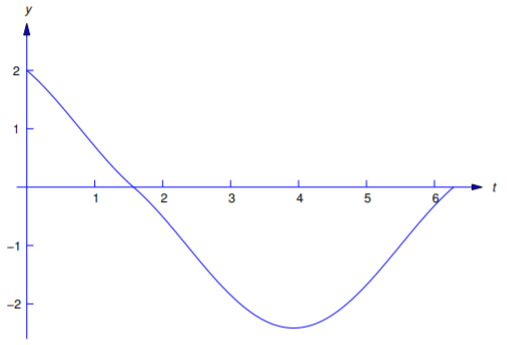
Resolver el problema de valor inicial
\[\label{eq:8.5.8} y''-y=f(t), \quad y(0)=-1,\; y'(0)=2,\]
donde
\[f(t)=\left\{\begin{array}{cl} t,&0\le t<1,\\ 1,&t\ge 1. \end{array}\right.\nonumber\]
Solución
Aquí
\[f(t)=t-u(t-1)(t-1),\nonumber\]
por lo
\[\begin{align*} {\cal L}(f)&={\cal L}(t)-{\cal L}\left(u(t-1)(t-1)\right)\\[4pt] &=\cal L(t)-e^{-s}{\cal L}(t)\text{ (from Theorem 8.4.1})\\[4pt] &={1\over s^2}-{e^{-s}\over s^2}.\end{align*}\nonumber\]
Desde la transformación de la ecuación\ ref {eq:8.5.8} rendimientos
\[(s^2-1) Y(s)={\cal L}(f)+2-s,\nonumber\]
vemos que
\[\label{eq:8.5.9} Y(s)=(1-e^{-s})H(s)+{2-s\over s^2-1},\]
donde
\[H(s)={1\over s^2(s^2-1)}={1\over s^2-1}-{1\over s^2};\nonumber\]
por lo tanto
\[\label{eq:8.5.10} h(t)=\sinh t-t.\]
Desde
\[{\cal L}^{-1}\left({2-s\over s^2-1}\right)=2\sinh t-\cosh t,\nonumber\]
concluimos de la Ecuación\ ref {eq:8.5.9}, Ecuación\ ref {eq:8.5.10}, y Teorema 8.5.1 que
\[y=\sinh t-t-u(t-1)\left(\sinh (t-1)-t+1\right)+2\sinh t- \cosh t,\nonumber\]
o
\[\label{eq:8.5.11} y=3\sinh t-\cosh t-t-u(t-1)\left(\sinh (t-1)-t+1\right)\]
Te dejamos a ti verificar eso\(y\) y\(y'\) son continuos y\(y''\) tiene límites desde la derecha y la izquierda en\(t_1=1\).
Resolver el problema de valor inicial
\[\label{eq:8.5.12} y''+y=f(t), \quad y(0)=0,\; y'(0)=0,\]
donde
\[f(t)=\left\{\begin{array}{cl}{0,}&{0\leq t<\frac{\pi }{4}}\\{\cos 2t}&{\frac{\pi }{4}\leq t< \pi }\\{0,}&{t\geq \pi } \end{array} \right.\nonumber \]
Solución
Aquí
\[f(t)=u(t-\pi/4)\cos2t-u(t-\pi)\cos2t, \nonumber\]
por lo
\[\begin{align*} {\cal L}(f)&={\cal L}\left(u(t-\pi/4)\cos2t\right)-{\cal L}\left( u(t-\pi)\cos2t\right)\\[4pt] &=e^{-{\pi s/4}}{\cal L}\left(\cos2(t+\pi/4)\right)-e^{-\pi s} {\cal L}\left(\cos2(t+\pi)\right)\\[4pt] &=-e^{-{\pi s/4}}{\cal L}(\sin2t)-e^{-\pi s} {\cal L}(\cos2t)\\[4pt] &=-{2e^{-{\pi s/ 4}}\over s^2+4}-{se^{-\pi s}\over s^2+4}.\end{align*}\nonumber\]
Desde la transformación de la ecuación\ ref {eq:8.5.12} rendimientos
\[(s^2+1)Y(s)={\cal L}(f),\nonumber\]
vemos que
\[\label{eq:8.5.13} Y(s)=e^{-{\pi s/ 4}} H_1(s)+e^{-\pi s} H_2(s),\]
donde
\[\label{eq:8.5.14} H_1(s)=-{2\over (s^2+1)(s^2+4)}\quad\mbox{ and }\quad H_2(s)=-{s \over (s^2+1)(s^2+4)}.\]
Para simplificar las expansiones de fracción parcial requeridas, primero escribimos
\[{1\over (x+1)(x+4)}={1\over3}\left[{1\over x+1}-{1\over x+4}\right].\nonumber\]
Establecer\(x=s^2\) y sustituir el resultado en Ecuación\ ref {eq:8.5.14} rendimientos
\[H_1(s)=-{2\over3}\left[{1\over s^2+1}-{1\over s^2+4}\right] \quad\mbox{ and }\quad H_2(s)=-{1\over3}\left[{s\over s^2+1}-{s\over s^2+4}\right].\nonumber\]
Las transformaciones inversas son
\[h_1(t)=-{2\over3}\sin t+{1\over3}\sin2t \quad\mbox{ and }\; h_2(t)=-{1\over3}\cos t+{1\over3}\cos2t.\nonumber\]
De la Ecuación\ ref {eq:8.5.13} y Teorema 8.4.2,
\[\label{eq:8.5.15} y=u\left(t-{\pi\over4}\right) h_1\left(t-{\pi\over4}\right)+ u(t-\pi) h_2(t-\pi).\]
Desde
\[\begin{aligned} h_1\left(t-{\pi\over4}\right)&=-{2\over3}\sin\left(t-{\pi\over 4}\right)+{1\over3}\sin2\left(t-{\pi\over4}\right)\\ &=-{\sqrt{2}\over3} (\sin t-\cos t)-{1\over3}\cos2t\end{aligned}\nonumber\]
y
\[\begin{align*} h_2(t-\pi)&=-{1\over3}\cos (t-\pi)+{1\over3}\cos2(t-\pi)\\ &={1\over3}\cos t+{1\over3}\cos2t,\end{align*}\nonumber\]
La ecuación\ ref {eq:8.5.15} se puede reescribir como
\[y=-{1\over3}u\left(t-{\pi\over4}\right)\left(\sqrt{2}(\sin t-\cos t)+\cos2t\right) + {1\over3} u(t-\pi) (\cos t+\cos2t)\nonumber\]
o
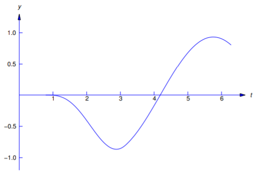
\[\label{eq:8.5.16} \left\{\begin{array}{cl}{0,}&{0\leq t< \frac{\pi }{4}}\\{-\frac{\sqrt{2}}{3}(\sin t-\cos t)-\frac{1}{3}\cos 2t,}&{\frac{\pi }{4}\leq t<\pi ,}\\{-\frac{\sqrt{2}}{3}\sin t+\frac{1+\sqrt{2}}{3}\cos t,}&{t\geq\pi } \end{array} \right. \]
Te dejamos a ti verificar eso\(y\) y\(y'\) son continuos y\(y''\) tiene límites de derecha e izquierda en\(t_1=\pi/4\) y\(t_2=\pi\) (Figura 8.5.2 ).