6.1: Fórmula de Poisson

Supongamos que\(u\) es una solución de (6.2), entonces, dado que la transformada de Fourier es un mapeo lineal,

\[\widehat{u_t-\triangle u}=\hat{0}.\]

De las propiedades de la transformada de Fourier, ver Proposición 5.1, tenemos

\[\widehat{\triangle u}=\sum_{k=1}^n\widehat{\frac{\partial^2 u}{\partial x_k^2}}=\sum_{k=1}^n i^2\xi^2_k\widehat{u}(\xi),\]

siempre que existan las transformaciones. Así llegamos a la ecuación diferencial ordinaria para la transformada de Fourier de\(u\)

\[\frac{d\widehat{u}}{dt}+|\xi|^2\widehat{u}=0,\]

donde\(\xi\) se considera como un parámetro. La solución es

\[\widehat{u}(\xi,t)=\widehat{\phi}(\xi)e^{-|\xi|^2 t}\]

ya que\(\widehat{u}(\xi,0)=\widehat{\phi}(\xi)\). Del Teorema 5.1 se sigue

\ begin {eqnarray*}
u (x, t) &=& (2\ pi) ^ {-n/2}\ int_ {\ mathbb {R} ^n}\\ sombrero ancho {\ phi} (\ xi) e^ {-|\ xi|^2t} e^ {i\ xi\ cdot x}\ d\ xi\
&=& (2\ pi) ^ {-^ -n}\ int_ {\ mathbb {R} ^n}\\ phi (y)\ izquierda (\ int_ {\ mathbb {R} ^n} e^ {i\ xi\ cdot (x-y) -|\ xi|^2t}\ d\ xi\ derecha)\ dy.
\ end {eqnarray*}

Set

$$K (x, y, t) = (2\ pi) ^ {-n}\ int_ {\ mathbb {R} ^n} e^ {i\ xi\ cdot (x-y) -|\ xi|^2t}\ d\ xi.\]

Por los mismos cálculos que en la prueba del Teorema 5.1, paso (vi), encontramos

\ begin {ecuación}
\ label {kernel1}
K (x, y, t) =( 4\ pi t) ^ {-n/2} e^ {-|x-y|^2/4t}.
\ end {ecuación}

\ (K (x, y, t)\),\(\rho=|x-y|\),\(t_1<t_2\) "height="213" width="403" src=” https://math.libretexts.org/@api/dek.../parabfig2.jpg "/>

Figura 6.1.1: Núcleo\(K(x,y,t)\),\(\rho=|x-y|\),\(t_1<t_2\)

Así tenemos

\ begin {ecuación}
\ label {poisson1}
u (x, t) =\ frac {1} {\ izquierda (2\ sqrt {\ pi t}\ derecha) ^n}\ int_ {\ mathbb {R} ^n}\ phi (z) e^ {-|x-z|^2/4t}\ dz.
\ end {ecuación}

Definición. La fórmula (\ ref {poisson1}) se llama fórmula de Poisson} y la función\(K\) definida por (\ ref {kernel1}) se llama núcleo de calor o solución fundamental de la ecuación de calor.

Proposición 6.1 El kernel\(K\) tiene las siguientes propiedades:

1. i)\(K(x,y,t)\in C^\infty(\mathbb{R}^n\times\mathbb{R}^n\times\mathbb{R}^1_+)\),
2. ii)\((\partial/\partial t\ -\triangle)K(x,y,t)=0,\ t>0\),
3. iii)\(K(x,y,t)>0,\ t>0\),
4. iv)\(\int_{\mathbb{R}^n}\ K(x,y,t)\ dy=1\) \(x\in\mathbb{R}^n\),\(t>0\)
5. \(\delta>0\):( v) Por cada fijo

$$\ lim_ {\ begin {array} {l} t\ to0\ t>0\ end {array}}\ int_ {\ mathbb {R} ^n\ setmenos B_\ delta (x)}\ K (x, y, t)\ dy=0$$

uniformemente para\(x\in\mathbb{R}\).

Comprobante. (i) y (iii) son obviamente, y (ii) se desprende de la definición de\(K\). Las ecuaciones (iv) y (v) se mantienen desde

\ begin {eqnarray*}
\ int_ {\ mathbb {R} ^n\ setmenos B_\ delta (x)}\ K (x, y, t)\ dy&=&\ int_ {\ mathbb {R} ^n\ setmenos B_\ delta (x)}\ (4\ pi t) ^ {-n/2} e^ {-|x-y|2/4t}\ dy\\
&=&\ pi^ {-n/2}\ int_ {\ mathbb {R} ^n\ setmenos B_ {\ delta/\ sqrt {4t}} (0)} e^ {-|\ eta|^2}\ d\ eta
\ end { eqnarray*}
mediante el uso de la sustitución\(y=x+(4t)^{1/2}\eta\). Para fijo\(\delta>0\) sigue (v) y para\(\delta:=0\) obtenemos (iv).

\(\Box\)

Teorema 6.1. Asumir\(\phi\in C(\mathbb{R}^n)\) y\(\sup_{\mathbb{R}^n}|\phi(x)|<\infty\). Entonces\(u(x,t)\) dada por la fórmula de Poisson (\ ref {poisson1}) está en\(C^{\infty}(\mathbb{R}^n\times\mathbb{R}^1_+)\), continua\(\mathbb{R}^n\times[0,\infty)\) y una solución del problema de valor inicial (6.2), (6.3).

Comprobante. Queda por mostrar

$$
\ lim_ {\ begin {array} {l} x\ to\ xi\
t\ to0\ end {array}} u (x, t) =\ phi (\ xi).
\]

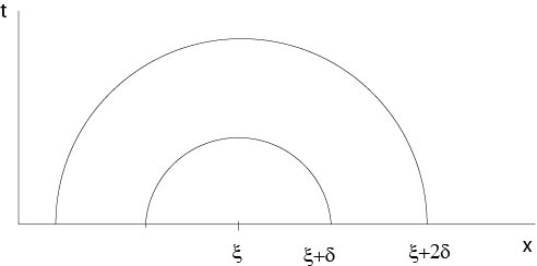
Figura 6.1.2: Figura a la prueba del Teorema 6.1

Ya que\(\phi\) es continuo existe para dado\(\varepsilon>0\) un\(\delta=\delta(\varepsilon)\) tal que\(|\phi(y)-\phi(\xi)|<\varepsilon\) si\(|y-\xi|<2\delta\).
Set\(M:=\sup_{\mathbb{R}^n}|\phi(y)|\). Entonces, ver Proposición 6.1,
$$
u (x, t) -\ phi (\ xi) =\ int_ {\ mathbb {R} ^n}\ K (x, y, t)\ izquierda (\ phi (y) -\ phi (\ xi)\ derecha)\ dy.
$$
Se deduce, si\(|x-\xi|<\delta\) y\(t>0\), que
\ begin {eqnarray*}
|u (x, t) -\ phi (\ xi) |&\ le&\ int_ {B_ {\ delta} (x)}\ K (x, y, t)\ izquierda|\ phi (y) -\ phi (\ xi)\ derecha|\ dy\
&&+\ int_ {\ mathbb {} ^n\ setmenos B_ {\ delta} (x)}\ K (x, y, t) \ izquierda|\ phi (y) -\ phi (\ xi)\ derecha|\ dy\
&\ le&\ int_ {B_ {2\ delta} (x)}\ K (x, y, t)\ izquierda|\ phi (y) -\ phi (\ xi)\ derecha|\ dy\
&&&+2M\ int_ {\ mathbb {R} ^n\ setmenos _ {\ delta} (x)}\ K (x, y, t)\ dy\\
&\ le&\ varepsilon\ int_ {\ mathbb {R} ^n}\ K (x, y, t)\ dy+2m\ int_ {\ mathbb {R} ^n\ setmenos B_ {\ delta} (x)}\ K (x, y, t)\ dy\\
&<&2\ varepsilon
\ end {eqnarray*}
si\(0<t\le t_0\),\(t_0\) suficientemente pequeño.

\(\Box\)

Observaciones. 1. La singularidad sigue bajo el supuesto de crecimiento adicional
$$
|u (x, t) |\ le Me^ {a|x|^2}\\\ mbox {in}\ D_T,
$$
donde\(M\) y\(a\) son constantes positivas,
vea la Proposición 6.2 a continuación.
En el caso unidimensional, uno tiene singularidad en la clase\(u(x,t)\ge 0\) en\(D_T\), ver [10], pp. 222.

2. \(u(x,t)\)definido por la fórmula de Poisson depende de todos los valores\(\phi(y)\),\(y\in\mathbb{R}^n\). Eso quiere decir, una perturbación de\(\phi\), incluso lejos de una fija\(x\), influye en el valor\(u(x,t)\). Esto significa que el calor viaja con una velocidad infinita, en contraste con la experiencia.

Colaboradores y Atribuciones

• Template:ContribMiersemann
• Template:ContribMarshall