7.2: Fórmula de representación

A continuación asumimos que\(\Omega\), la función\(\phi\) que aparece en la definición de la solución fundamental y la función potencial\(u\) considerada son suficientemente regulares como para que los siguientes cálculos tengan sentido, véase [6] para generalizaciones. Este es el caso si\(\Omega\) está acotado,\(\partial\Omega\) está en\(C^1\),\(\phi\in C^2(\overline{\Omega})\) para cada fijo\(y\in\Omega\) y\(u\in C^2(\overline{\Omega})\).

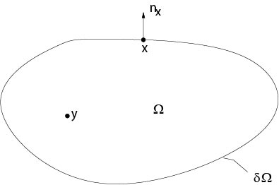
Figura 7.2.1: Notaciones a la identidad de Green

Teorema 7.1. Dejar\(u\) ser una función potencial y\(\gamma\) una solución fundamental, entonces para cada fijo\(y\in\Omega\)
$$
u (y) =\ int_ {\ parcial\ Omega}\ left (\ gamma (x, y)\ frac {\ parcial u (x)} {\ parcial n_x} -u (x)\ frac {\ parcial\ gamma (x, y)} {\ parcial n_x}\ derecha)\ ds_x.
$$

Prueba. Que\(B_\rho(y)\subset\Omega\) sea una pelota. Set\(\Omega_\rho(y)=\Omega\setminus B_\rho(y)\). Consulte la Figura 7.2.2 para las anotaciones.

Figura 7.2.2: Notaciones al teorema 7.1

De la fórmula de Green, para\(u,\ v\in C^2(\overline{\Omega})\),
$$
\ int_ {\ Omega_\ rho (y)}\ (v\ triángulo u-u\ triángulo v)\ dx=\ int_ {\ parcial\ Omega_\ rho (y)}\\ izquierda (v\ frac {\ parcial u} {\ parcial n} -u\ frac {\ parcial v} {\ parcial n}\ derecha)\ dS
$$
nosotros obtener, si\(v\) es fundamental solución y\(u\) una función potencial,
$$
\ int_ {\ parcial\ Omega_\ rho (y)}\\ izquierda (v\ frac {\ parcial u} {\ parcial n} -u\ frac {\ v parcial} {\ parcial n}\ derecha)\ ds=0.
$$
Así tenemos que considerar
\ begin {eqnarray*}
\ int_ {\ parcial\ Omega_ {\ rho} (y)}\ v\ frac {\ parcial u} {\ parcial n}\ ds&=&\ int_ {\ parcial\ Omega}\ v\ frac {\ parcial u} {\ parcial n}\ dS+\ int_ {\ parcial B_\ rho y ()}\ v\ frac {\ u parcial} {\ parcial n}\ dS\\
\ int_ {\ parcial\ Omega_ {\ rho} (y)}\ u\ frac {\ parcial v} {\ parcial n}\ dS&=&\ int_ {\ parcial\ Omega}\ u\ frac {\ parcial v} {\ parcial n}\ dS+\ int_ {\ parcial B_\ rho (y)}\ u\ frac {\ parcial v} {parcial\ n}\ dS.
\ end {eqnarray*}
Estimamos las integrales sobre\(\partial B_\rho(y)\):

(i)
\ begin {eqnarray*}
\ izquierda|\ int_ {\ parcial B_\ rho (y)}\ v\ frac {\ parcial u} {\ parcial n}\ dS\ derecha|&\ le&M\ int_ {\ parcial B_\ rho (y)}\ |v|\ dS\
&\ Le&M\ izquierda (\ int_ {\ parcial B_\ rho (y)}\ s (\ rho)\ dS+c\ omega_n\ rho^ {n-1}\ derecha),
\ fin {eqnarray*}
donde
\ begin {eqnarray*}
M&=&M (y) =\ sup_ {B_ {\ rho_0} (y)} |\ parcial u/\ parcial n|,\\\ rho\ le\ rho_0,\\
C&=&C (y) =\ sup_ {x\ in B_ {\ rho_0} (y)} |\ phi (x, y) |.
\ end {eqnarray*}
De la definición de\(s(\rho)\) obtenemos la estimación como\(\rho\to 0\)
\ begin {ecuación}
\ label {ell1}
\ int_ {\ parcial B_\ rho (y)}\ v\ frac {\ parcial u} {\ parcial n}\ ds=\ left\ {\ begin {array} {r@ {\ qua d:\quad} l}
O (\ rho|\ ln\ rho|) &n=2\\
O (\ rho) &n\ ge3.
\ end {array}\ right.
\ end {ecuación}

(ii) Considerar el caso\(n\ge3\), entonces
\ comenzar {eqnarray*}
\ int_ {\ parcial B_\ rho (y)}\ u\ frac {\ parcial v} {\ parcial n}\ ds&=&
\ frac {1} {\ omega_n}\ int_ {\ parcial B_\ rho (y)}\ u\ frac {1} {\ rho^ {n-1}}\ dS+\ int_ {\ parcial B_\ rho (y)}\ u\ frac {\ parcial\ phi} {\ parcial n}\ dS\\
&=&\ frac {1} {\ omega_n\ rho^ {n-1}}\ int_ {\ parcial B_\ rho (y)}\ u\ dS+o (\ rho^ {n-1})\\
&=&\ frac {1} {\ omega_n\ rho^ {n-1}} u (x_0)\ int_ {\ parcial B_\ rho (y)}\ dS+o (\ rho^ {n-1}),\\ &=&u (x_0) +O (\ rho^ {n-1}).
\ end {eqnarray*}
para un\(x_0\in\partial B_\rho(y)\).

Combinando esta estimación y (\ ref {ell1}), obtenemos la fórmula de representación del teorema.

\(\Box\)

Corolario. Establecer\(\phi\equiv 0\) y\(r=|x-y|\) en la fórmula de representación del Teorema 7.1, entonces
\ begin {eqnarray}
\ label {ell2}
u (y) &=&\ frac {1} {2\ pi}\ int_ {\ parcial\ Omega}\\ izquierda (\ ln r\ frac {\ parcial u} {\ parcial n_x} -u\ frac {\ parcial (\ ln r)} {\ parcial n__x}\ derecha)\ DS_x,\\ n =2,\\
\ etiqueta {ell3}
u (y) &=&\ frac {1} {(n-2)\ omega_n}\ int_ {\ parcial\ Omega}\\ izquierda (\ frac {1} {r^ {n-2}}\ frac {\ u parcial} {\ parcial n_x} -u\ frac {\ parcial (r^ {2-n})}\ parcial n_x}\ derecha)\ DS_x,\\ n\ ge3.
\ end {eqnarray}

Colaboradores y Atribuciones

• Template:ContribMiersemann
• Template:ContribMarshall