Saltar al contenido principal
LibreTexts Español

7.1: Coordenadas polares

  • Page ID
    113827
  • \( \newcommand{\vecs}[1]{\overset { \scriptstyle \rightharpoonup} {\mathbf{#1}} } \)

    \( \newcommand{\vecd}[1]{\overset{-\!-\!\rightharpoonup}{\vphantom{a}\smash {#1}}} \)

    \( \newcommand{\id}{\mathrm{id}}\) \( \newcommand{\Span}{\mathrm{span}}\)

    ( \newcommand{\kernel}{\mathrm{null}\,}\) \( \newcommand{\range}{\mathrm{range}\,}\)

    \( \newcommand{\RealPart}{\mathrm{Re}}\) \( \newcommand{\ImaginaryPart}{\mathrm{Im}}\)

    \( \newcommand{\Argument}{\mathrm{Arg}}\) \( \newcommand{\norm}[1]{\| #1 \|}\)

    \( \newcommand{\inner}[2]{\langle #1, #2 \rangle}\)

    \( \newcommand{\Span}{\mathrm{span}}\)

    \( \newcommand{\id}{\mathrm{id}}\)

    \( \newcommand{\Span}{\mathrm{span}}\)

    \( \newcommand{\kernel}{\mathrm{null}\,}\)

    \( \newcommand{\range}{\mathrm{range}\,}\)

    \( \newcommand{\RealPart}{\mathrm{Re}}\)

    \( \newcommand{\ImaginaryPart}{\mathrm{Im}}\)

    \( \newcommand{\Argument}{\mathrm{Arg}}\)

    \( \newcommand{\norm}[1]{\| #1 \|}\)

    \( \newcommand{\inner}[2]{\langle #1, #2 \rangle}\)

    \( \newcommand{\Span}{\mathrm{span}}\) \( \newcommand{\AA}{\unicode[.8,0]{x212B}}\)

    \( \newcommand{\vectorA}[1]{\vec{#1}}      % arrow\)

    \( \newcommand{\vectorAt}[1]{\vec{\text{#1}}}      % arrow\)

    \( \newcommand{\vectorB}[1]{\overset { \scriptstyle \rightharpoonup} {\mathbf{#1}} } \)

    \( \newcommand{\vectorC}[1]{\textbf{#1}} \)

    \( \newcommand{\vectorD}[1]{\overrightarrow{#1}} \)

    \( \newcommand{\vectorDt}[1]{\overrightarrow{\text{#1}}} \)

    \( \newcommand{\vectE}[1]{\overset{-\!-\!\rightharpoonup}{\vphantom{a}\smash{\mathbf {#1}}}} \)

    \( \newcommand{\vecs}[1]{\overset { \scriptstyle \rightharpoonup} {\mathbf{#1}} } \)

    \( \newcommand{\vecd}[1]{\overset{-\!-\!\rightharpoonup}{\vphantom{a}\smash {#1}}} \)

    \(\newcommand{\avec}{\mathbf a}\) \(\newcommand{\bvec}{\mathbf b}\) \(\newcommand{\cvec}{\mathbf c}\) \(\newcommand{\dvec}{\mathbf d}\) \(\newcommand{\dtil}{\widetilde{\mathbf d}}\) \(\newcommand{\evec}{\mathbf e}\) \(\newcommand{\fvec}{\mathbf f}\) \(\newcommand{\nvec}{\mathbf n}\) \(\newcommand{\pvec}{\mathbf p}\) \(\newcommand{\qvec}{\mathbf q}\) \(\newcommand{\svec}{\mathbf s}\) \(\newcommand{\tvec}{\mathbf t}\) \(\newcommand{\uvec}{\mathbf u}\) \(\newcommand{\vvec}{\mathbf v}\) \(\newcommand{\wvec}{\mathbf w}\) \(\newcommand{\xvec}{\mathbf x}\) \(\newcommand{\yvec}{\mathbf y}\) \(\newcommand{\zvec}{\mathbf z}\) \(\newcommand{\rvec}{\mathbf r}\) \(\newcommand{\mvec}{\mathbf m}\) \(\newcommand{\zerovec}{\mathbf 0}\) \(\newcommand{\onevec}{\mathbf 1}\) \(\newcommand{\real}{\mathbb R}\) \(\newcommand{\twovec}[2]{\left[\begin{array}{r}#1 \\ #2 \end{array}\right]}\) \(\newcommand{\ctwovec}[2]{\left[\begin{array}{c}#1 \\ #2 \end{array}\right]}\) \(\newcommand{\threevec}[3]{\left[\begin{array}{r}#1 \\ #2 \\ #3 \end{array}\right]}\) \(\newcommand{\cthreevec}[3]{\left[\begin{array}{c}#1 \\ #2 \\ #3 \end{array}\right]}\) \(\newcommand{\fourvec}[4]{\left[\begin{array}{r}#1 \\ #2 \\ #3 \\ #4 \end{array}\right]}\) \(\newcommand{\cfourvec}[4]{\left[\begin{array}{c}#1 \\ #2 \\ #3 \\ #4 \end{array}\right]}\) \(\newcommand{\fivevec}[5]{\left[\begin{array}{r}#1 \\ #2 \\ #3 \\ #4 \\ #5 \\ \end{array}\right]}\) \(\newcommand{\cfivevec}[5]{\left[\begin{array}{c}#1 \\ #2 \\ #3 \\ #4 \\ #5 \\ \end{array}\right]}\) \(\newcommand{\mattwo}[4]{\left[\begin{array}{rr}#1 \amp #2 \\ #3 \amp #4 \\ \end{array}\right]}\) \(\newcommand{\laspan}[1]{\text{Span}\{#1\}}\) \(\newcommand{\bcal}{\cal B}\) \(\newcommand{\ccal}{\cal C}\) \(\newcommand{\scal}{\cal S}\) \(\newcommand{\wcal}{\cal W}\) \(\newcommand{\ecal}{\cal E}\) \(\newcommand{\coords}[2]{\left\{#1\right\}_{#2}}\) \(\newcommand{\gray}[1]{\color{gray}{#1}}\) \(\newcommand{\lgray}[1]{\color{lightgray}{#1}}\) \(\newcommand{\rank}{\operatorname{rank}}\) \(\newcommand{\row}{\text{Row}}\) \(\newcommand{\col}{\text{Col}}\) \(\renewcommand{\row}{\text{Row}}\) \(\newcommand{\nul}{\text{Nul}}\) \(\newcommand{\var}{\text{Var}}\) \(\newcommand{\corr}{\text{corr}}\) \(\newcommand{\len}[1]{\left|#1\right|}\) \(\newcommand{\bbar}{\overline{\bvec}}\) \(\newcommand{\bhat}{\widehat{\bvec}}\) \(\newcommand{\bperp}{\bvec^\perp}\) \(\newcommand{\xhat}{\widehat{\xvec}}\) \(\newcommand{\vhat}{\widehat{\vvec}}\) \(\newcommand{\uhat}{\widehat{\uvec}}\) \(\newcommand{\what}{\widehat{\wvec}}\) \(\newcommand{\Sighat}{\widehat{\Sigma}}\) \(\newcommand{\lt}{<}\) \(\newcommand{\gt}{>}\) \(\newcommand{\amp}{&}\) \(\definecolor{fillinmathshade}{gray}{0.9}\)

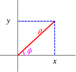
    Las coordenadas polares en dos dimensiones se definen\[\begin{aligned} x = \rho\cos\phi, y= \rho\sin\phi,\\ \rho = \sqrt{x^2+y^2}, \phi = \arctan(y/x),\end{aligned} \nonumber \] como se indica esquemáticamente en la Fig. \(\PageIndex{1}\).

    polar.png
    Figura\(\PageIndex{1}\): Coordenadas polares

    Usando la regla de la cadena encontramos

    \[\begin{aligned} \frac{\partial}{\partial x}{~} &= \frac{\partial \rho}{\partial x}\frac{\partial}{\partial \rho}{~}+\frac{\partial \phi}{\partial x}\frac{\partial}{\partial \phi}{~}\nonumber\\ &= \frac{x}{\rho}\frac{\partial}{\partial \rho}{~}-\frac{y}{\rho^2}\frac{\partial}{\partial \phi}{~}\nonumber\\ &= \cos\phi\frac{\partial}{\partial \rho}{~}-\frac{\sin\phi}{\rho}\frac{\partial}{\partial \phi}{~},\\ \frac{\partial}{\partial y}{~} &= \frac{\partial \rho}{\partial y}\frac{\partial}{\partial \rho}{~}+\frac{\partial \phi}{\partial y}\frac{\partial}{\partial \phi}{~}\nonumber\\ &= \frac{y}{\rho}\frac{\partial}{\partial \rho} {~}+\frac{x}{\rho^2}\frac{\partial}{\partial \phi}{~}\nonumber\\ &= \sin\phi\frac{\partial}{\partial \rho}{~}+\frac{\cos\phi}{\rho}\frac{\partial}{\partial \phi}{~},\end{aligned} \nonumber \]Podemos escribir\[\begin{aligned} {\nabla} &= {\hat{e}}_\rho \frac{\partial}{\partial \rho}{~}+\hat{e}_\phi \frac{1}{\rho} \frac{\partial}{\partial \phi}{~}\end{aligned} \nonumber \]

    donde los vectores unitarios

    \[\begin{aligned} \hat{e}_\rho &= (\cos\phi,\sin\phi), \nonumber\\ \hat{e}_\phi &= (-\sin\phi,\cos\phi), \end{aligned} \nonumber \]son un conjunto ortonormal. Decimos que las coordenadas circulares son ortogonales.

    Ahora podemos usar esto para evaluar\(\nabla^2\),

    \[\begin{aligned} \nabla^2 &= \cos^2\phi\frac{\partial^2}{\partial \rho^2}{~} + \frac{\sin\phi\cos\phi}{\rho^2}\frac{\partial}{\partial \phi} {~} +\frac{\sin^2\phi}{\rho}\frac{\partial}{\partial \rho} {~} + \frac{\sin^2\phi}{\rho^2}\frac{\partial^2}{\partial \phi^2} {~} + \frac{\sin\phi\cos\phi}{\rho^2} \frac{\partial}{\partial \phi} {~}\nonumber\\ &\space\space\space+\sin^2\phi\frac{\partial^2}{\partial \rho^2} {~}-\frac{\sin\phi\cos\phi}{\rho^2}\frac{\partial}{\partial \phi} {~} +\frac{\cos^2\phi}{\rho}\frac{\partial}{\partial \rho} {~} + \frac{\cos^2\phi}{\rho^2}\frac{\partial^2}{\partial \phi^2} {~} - \frac{\sin\phi\cos\phi}{\rho^2} \frac{\partial}{\partial \phi}{~}\\ &=\frac{\partial^2}{\partial \rho^2} {~} +\frac{1}{\rho}\frac{\partial}{\partial \rho}{~} + \frac{1}{\rho^2}\frac{\partial^2}{\partial \phi^2} {~}\nonumber\\ &=\frac{1}{\rho}\frac{\partial}{\partial \rho} {~} \left(\rho\frac{\partial}{\partial \rho} {~}\right) +\frac{1}{\rho^2}\frac{\partial^2}{\partial \phi^2} {~}.\nonumber\\\end{aligned} \nonumber \]

    Una relación útil final es la integración sobre estas coordenadas.

    imageedit_2_5805175308.png
    Figura\(\PageIndex{2}\): Integración en coordenadas polares

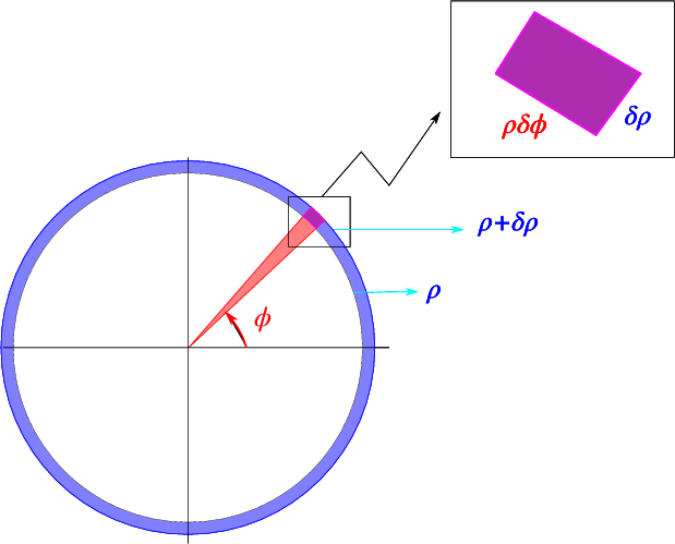
    Como se indica esquemáticamente en la Fig. \(\PageIndex{2}\), la superficie relacionada con un cambio\(\rho \rightarrow \rho + \delta \rho\),\(\phi \rightarrow \phi+\delta\phi\) es\(\rho \delta \rho \delta\phi\). Esto nos lleva a la conclusión de que una integral sobre\(x,y\) puede reescribirse como\[\int_V f(x,y) dx dy = \int_V f(\rho\cos\phi,\rho\sin\phi) \rho \,d\rho\, d\phi \nonumber \]


    This page titled 7.1: Coordenadas polares is shared under a CC BY-NC-SA 2.0 license and was authored, remixed, and/or curated by Niels Walet via source content that was edited to the style and standards of the LibreTexts platform.