11.4: Modelado del ojo—revisitado

Última actualización
Guardar como PDF

Page ID: 113742

$ \newcommand{\vecs}[1]{\overset { \scriptstyle \rightharpoonup} {\mathbf{#1}} } $ $ \newcommand{\vecd}[1]{\overset{-\!-\!\rightharpoonup}{\vphantom{a}\smash {#1}}} $$\newcommand{\id}{\mathrm{id}}$ $ \newcommand{\Span}{\mathrm{span}}$ $ \newcommand{\kernel}{\mathrm{null}\,}$ $ \newcommand{\range}{\mathrm{range}\,}$ $ \newcommand{\RealPart}{\mathrm{Re}}$ $ \newcommand{\ImaginaryPart}{\mathrm{Im}}$ $ \newcommand{\Argument}{\mathrm{Arg}}$ $ \newcommand{\norm}[1]{\| #1 \|}$ $ \newcommand{\inner}[2]{\langle #1, #2 \rangle}$ $ \newcommand{\Span}{\mathrm{span}}$ $\newcommand{\id}{\mathrm{id}}$ $ \newcommand{\Span}{\mathrm{span}}$ $ \newcommand{\kernel}{\mathrm{null}\,}$ $ \newcommand{\range}{\mathrm{range}\,}$ $ \newcommand{\RealPart}{\mathrm{Re}}$ $ \newcommand{\ImaginaryPart}{\mathrm{Im}}$ $ \newcommand{\Argument}{\mathrm{Arg}}$ $ \newcommand{\norm}[1]{\| #1 \|}$ $ \newcommand{\inner}[2]{\langle #1, #2 \rangle}$ $ \newcommand{\Span}{\mathrm{span}}$$\newcommand{\AA}{\unicode[.8,0]{x212B}}$

Déjame volver a mi modelo de ojo. Con la función$P_n(\cos\theta)$ como solución a la ecuación angular, encontramos que las soluciones a la ecuación radial son

\[R=Ar^n + Br^{-n-1}. \nonumber \]

La parte singular no es aceptable, por lo que una vez más encontramos que la solución toma la forma

\[u(r,\theta) = \sum_{n=0}^\infty A_n r^n P_n(\cos\theta) \nonumber \]

Ahora necesitamos imponer la condición límite de que la temperatura es$20^\circ$ C en un ángulo de apertura de$45^\circ$, y en$36^\circ$ otros lugares. Esto lleva a la ecuación

\[\begin{aligned} \sum_{n=0}^\infty A_n c^n P_n(\cos\theta) = \left\{ \begin{array}{ll} 20 & 0<\theta<\pi/4\\ 36 & \pi/4 < \theta < \pi \end{array}\right.\end{aligned} \nonumber \]

Esto lleva a la integral, después de cambiar una vez más a$x=\cos\theta$,

\[A_n = \frac{2n+1}{2} \left[\int_{-1}^1 36 P_n(x) dx -\int_{\frac{1}{2}\sqrt{2}}^1 16 P_n(x) dx\right]. \nonumber \]

Estas integrales se pueden evaluar fácilmente, y se puede encontrar un boceto para la temperatura en la figura$\PageIndex{1}$.

$eye.png$

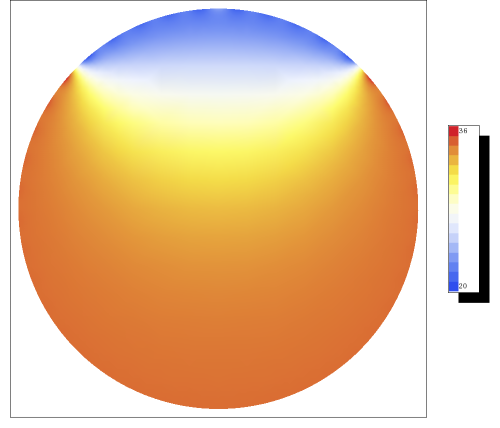
Figura$\PageIndex{1}$: Una sección transversal de la temperatura en el ojo. Hemos resumido los primeros 40 polinomios de Legendre.

Observe que necesitamos integrarnos sobre$x=\cos\theta$ para obtener los coeficientes$A_n$. La integración sobre$\theta$ en coordenadas esféricas es$\int_0^\pi \sin \theta d\theta = \int_{-1}^1 1 dx$, y así automáticamente implica que$\cos\theta$ es la variable correcta a usar, como también se desprende de la ortogonalidad de$P_n(x)$.