
6.2.1: Sistemas Masa-Muelle
- Page ID
- 119622

LOS PRIMEROS EJEMPLOS QUE HABÍAMOS VISTO involucraban masas sobre Recordemos que para una masa simple en un resorte estudiamos el movimiento armónico simple, que se rige por la ecuación
\[m \ddot{x}+k x=0\nonumber \]
Esta ecuación de segundo orden se puede escribir como dos ecuaciones de primer orden
\[\begin{array}{r} \dot{x}=y \\ \dot{y}=-\dfrac{k}{m} x \end{array} \nonumber \]
o
\[\begin{array}{r} \dot{x}=y \\ \dot{y}=-\omega^{2} x \end{array} \nonumber \]
donde\(\omega^{2}=\dfrac{k}{m}\). La matriz de coeficientes para este sistema es
\[A=\left(\begin{array}{cc} 0 & 1 \\ -\omega^{2} & 0 \end{array}\right) \nonumber \]
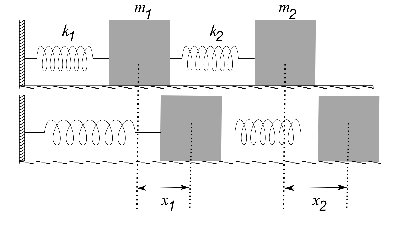
También observamos el sistema de dos masas y dos muelles como se muestra en la Figura\(6.20\). Las ecuaciones que rigen el movimiento de las masas es
\[ \begin{aligned} &m_{1} \ddot{x}_{1}=-k_{1} x_{1}+k_{2}\left(x_{2}-x_{1}\right) \\ &m_{2} \ddot{x}_{2}=-k_{2}\left(x_{2}-x_{1}\right) \end{aligned} \label{6.40} \]
Podemos reescribir este sistema como cuatro ecuaciones de primer orden
\[ \begin{aligned} \dot{x}_{1} &=x_{3} \\ \dot{x}_{2} &=x_{4} \\ \dot{x}_{3} &=-\dfrac{k_{1}}{m_{1}} x_{1}+\dfrac{k_{2}}{m_{1}}\left(x_{2}-x_{1}\right) \\ \dot{x}_{4} &=-\dfrac{k_{2}}{m_{2}}\left(x_{2}-x_{1}\right) \end{aligned} \label{6.41} \]
La matriz de coeficientes para este sistema es
\ [A=\ left (\ begin {array} {cccc}
0 & 0 & 1 & 0\\
0 & 0 & 0 & 0 & 1\\
-\ dfrac {k_ {1} +k_ {2}} {m_ {1}} &\ dfrac {k_ {2}} {m_ {1}} & 0\\
\ dfrac {k_ {2}} {m_ {2}} & -\ dfrac {k_ {2}} {m_ {2}} & 0 & 0
\ end {array}\ derecha)\ nonumber\]
Podemos estudiar este sistema para valores específicos de las constantes utilizando los métodos cubiertos en las últimas secciones.
Escribir el sistema de bloque de resorte como un sistema vectorial de segundo orden.
\ [\ left (\ begin {array} {cc}
m_ {1} & 0\\
0 & m_ {2}
\ end {array}\ right)\ left (\ begin {array} {c}
\ ddot {x} _ {1}\
\ ddot {x} _ {2}
\ end {array}\ right) =\ left (\ begin {array} {cc}
-\ left (k_ {1} +k_ {2}\ derecha) & k_ {2}\ \
k_ {2} & -k_ {2}
\ end {array}\ right)\ left (\ begin {array} {l}
x_ {1}\\
x_ {2}
\ end {array}\ right). \ nonumber\]
Este sistema se puede escribir de forma compacta como
\[ M \ddot{\mathbf{x}}=-K \mathbf{x}, \nonumber \]
donde
\[M=\left(\begin{array}{cc} m_{1} & 0 \\ 0 & m_{2} \end{array}\right), \quad K=\left(\begin{array}{cc} k_{1}+k_{2} & -k_{2} \\ -k_{2} & k_{2} \end{array}\right) \nonumber \]
Este sistema se puede resolver adivinando un formulario para la solución. Podríamos adivinar
\[\mathbf{x}=\mathbf{a} e^{i \omega t} \nonumber \]
O
\[\mathbf{x}=\left(\begin{array}{l} a_{1} \cos \left(\omega t-\delta_{1}\right) \\ a_{2} \cos \left(\omega t-\delta_{2}\right) \end{array}\right)\nonumber \]
donde\(\delta_{i}\) se determinan los desplazamientos de fase a partir de las condiciones iniciales.
La\(\mathbf{x}=\mathbf{a} e^{i \omega t}\) inserción en el sistema da
\[\left(K-\omega^{2} M\right) \mathbf{a}=\mathbf{0} \nonumber \]
Este es un sistema homogéneo. Es un problema generalizado de valores propios para valores propios\(\omega^{2}\) y vectores propios a, lo resolvemos de manera similar a los problemas de valores propios de la matriz estándar. La ecuación del valor propio se encuentra como
\[\operatorname{det}\left(K-\omega^{2} M\right)=0\nonumber \]
Una vez que se encuentran los valores propios, se determinan los vectores propios y se construye la solución.
Dejar\(m_{1}=m_{2}=m\) y\(k_{1}=k_{2}=k\). Entonces, tenemos que resolver el sistema
\[\omega^{2}\left(\begin{array}{cc} m & 0 \\ 0 & m \end{array}\right)\left(\begin{array}{l} a_{1} \\ a_{2} \end{array}\right)=\left(\begin{array}{cc} 2 k & -k \\ -k & k \end{array}\right)\left(\begin{array}{l} a_{1} \\ a_{2} \end{array}\right)\nonumber \]
La ecuación del valor propio viene dada por
\[ \begin{aligned} 0 &=\left|\begin{array}{cc} 2 k-m \omega^{2} & -k \\ -k & k-m \omega^{2} \end{array}\right| \\ &=\left(2 k-m \omega^{2}\right)\left(k-m \omega^{2}\right)-k^{2} \\ &=m^{2} \omega^{4}-3 k m \omega^{2}+k^{2} \end{aligned} \label{6.44} \]
Resolviendo esta ecuación cuadrática para\(\omega^{2}\), tenemos
\[\omega^{2}=\dfrac{3 \pm 1}{2} \dfrac{k}{m}\nonumber \]
Para valores positivos de\(\omega\), se puede demostrar que
\[\omega=\dfrac{1}{2}(\pm 1+\sqrt{5}) \sqrt{\dfrac{k}{m}}\nonumber \]
Los vectores propios se pueden encontrar para cada valor propio resolviendo el sistema homogéneo
\[\left(\begin{array}{cc} 2 k-m \omega^{2} & -k \\ -k & k-m \omega^{2} \end{array}\right)\left(\begin{array}{c} a_{1} \\ a_{2} \end{array}\right)=0\nonumber \]
Los vectores propios vienen dados por
\[\mathbf{a}_{1}=\left(\begin{array}{c} -\dfrac{\sqrt{5}+1}{2} \\ 1 \end{array}\right), \quad \mathbf{a}_{2}=\left(\begin{array}{c} \dfrac{\sqrt{5}-1}{2} \\ 1 \end{array}\right)\nonumber \]
Ahora estamos listos para construir las soluciones reales al problema. Similar a resolver dos sistemas de primer orden con raíces complejas, tomamos las partes real e imaginaria y tomamos una combinación lineal de las soluciones. En este problema hay cuatro términos, dando la solución en la forma
\[\mathbf{x}(t)=c_{1} \mathbf{a}_{1} \cos \omega_{1} t+c_{2} \mathbf{a}_{1} \sin \omega_{1} t+c_{3} \mathbf{a}_{2} \cos \omega_{2} t+c_{4} \mathbf{a}_{2} \sin \omega_{2} t\nonumber \]
donde\(\omega^{\prime}\) s son los valores propios y los a's son los vectores propios correspondientes. Las constantes se determinan a partir de las condiciones iniciales,\(\mathbf{x}(0)=\mathbf{x}_{0}\) y\(\dot{\mathbf{x}}(0)=\mathbf{v}_{0} .\)