8.5: Soluciones para el Capítulo 5

Última actualización
Guardar como PDF

Page ID: 112220

$ \newcommand{\vecs}[1]{\overset { \scriptstyle \rightharpoonup} {\mathbf{#1}} } $ $ \newcommand{\vecd}[1]{\overset{-\!-\!\rightharpoonup}{\vphantom{a}\smash {#1}}} $$\newcommand{\id}{\mathrm{id}}$ $ \newcommand{\Span}{\mathrm{span}}$ $ \newcommand{\kernel}{\mathrm{null}\,}$ $ \newcommand{\range}{\mathrm{range}\,}$ $ \newcommand{\RealPart}{\mathrm{Re}}$ $ \newcommand{\ImaginaryPart}{\mathrm{Im}}$ $ \newcommand{\Argument}{\mathrm{Arg}}$ $ \newcommand{\norm}[1]{\| #1 \|}$ $ \newcommand{\inner}[2]{\langle #1, #2 \rangle}$ $ \newcommand{\Span}{\mathrm{span}}$ $\newcommand{\id}{\mathrm{id}}$ $ \newcommand{\Span}{\mathrm{span}}$ $ \newcommand{\kernel}{\mathrm{null}\,}$ $ \newcommand{\range}{\mathrm{range}\,}$ $ \newcommand{\RealPart}{\mathrm{Re}}$ $ \newcommand{\ImaginaryPart}{\mathrm{Im}}$ $ \newcommand{\Argument}{\mathrm{Arg}}$ $ \newcommand{\norm}[1]{\| #1 \|}$ $ \newcommand{\inner}[2]{\langle #1, #2 \rangle}$ $ \newcommand{\Span}{\mathrm{span}}$$\newcommand{\AA}{\unicode[.8,0]{x212B}}$

Ejercicio 5.5

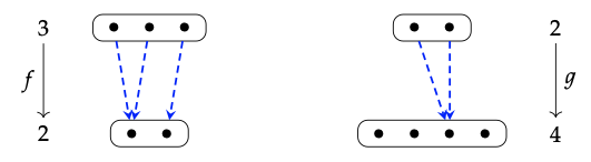
1. A continuación dibujamos un morfismo f: 3 → 2 y un morfismo g: 2 → 4 en FinSet:

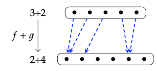
$Screen Shot 2021-02-09 en 2.45.51 PM.png$

2. Aquí hay una imagen de f + g

$Screen Shot 2021-02-09 en 2.46.31 PM.png$

El compuesto de morfismos f: m → n y g: n → p en FinSet es la función (f; g): m → p dada por (f; g) (i) = g (f (i)) para todos 1 ≤ i ≤ m.
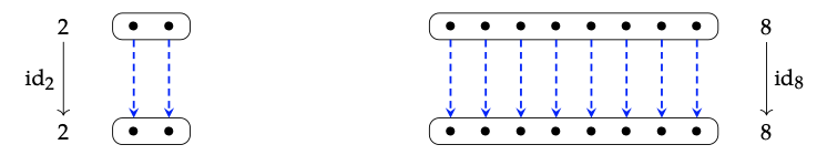
La identidad id$_{m}$: m → m viene dada por id$_{m}$ (i) = i para todos 1 ≤ i ≤ m. Aquí hay una foto de id$_{2}$ e id$_{8}$:

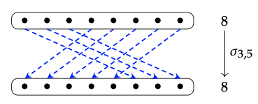
$Screen Shot 2021-02-09 en 2.47.12 PM.png$

5. Aquí hay una imagen de la simetría σ$_{3,5}$: 8 → 8:

$Screen Shot 2021-02-09 en 2.47.40 PM.png$

Ejercicio 5.9

Necesitamos dar ejemplos de apoyos posetales, es decir, cada uno será un poset cuyo conjunto de objetos es N, cuyo orden se denota m$\leq$ n, y con la propiedad

que siempre que m$_{1}$$\leq$ n$_{1}$ y m$_{2}$$\leq$ n se$_{2}$ mantengan entonces m$_{1}$ + m$_{2}$$\leq$ n$_{1}$ + n también$_{2}$ lo hace.

La pregunta sólo pide tres, pero además daremos un cuasi-ejemplo y un no-ejemplo.

1. Tomar$\leq$ para ser el orden discreto: m$\leq$ n iff m = n.

2. Toma$\leq$ para ser el orden habitual, m$\leq$ n iff existe d$\in$ N con d + m = n.

3. Toma$\leq$ para estar ahí verso del orden habitual, m$\leq$ n iff existe d$\in$ N con m = n + d.

4. Tomar$\leq$ para ser el orden co-discreto m $\leq$n para todos m, n. Algunos pueden objetar que esto es un preorden, no un poset, así que lo llamamos cuasi-ejemplo.

5. (No ejemplo.) Toma$\leq$ para ser el orden de división, m$\leq$ n iff existe q$\in$ N con m ∗ q = d. Este es un poset perfectamente bueno, pero no satisface la propiedad de monotonicidad: tenemos 2$\leq$ 4 y 3$\leq$ 3 pero no 5$\leq$$^{?}$ 7.

Ejercicio 5.10

Ejemplo 5.6: El prop Bij tiene

1. Bij (m, n) := {f:$\underline{m}$ →$\underline{n}$ | f es una biyección}. Tenga en cuenta que Bij (m, n) = Ø si m$\neq$ n y tiene n! elementos si m = n.

2. El mapa de identidad n → n es la biyección$\underline{n}$ →$\underline{n}$ enviando i → i.

3.El mapa de simetría m$\underline{n}$ +$\underline{n}$ → + m es la biyección σ$_{m, n}$:$\underline{m + n}$ →$\underline{n + m}$ dada por

$Screen Shot 2021-02-09 a las 6.30.10 PM.png$

4. Composición de las bijecciones m → n y n → p es solo su composición como funciones, que de nuevo es una bijección.

5. Dadas las biyecciones f: m → m ′ y g: n → n ′, su producto monoidal (f+ g): (m + n) → (m ′ + n ′) viene dado por

$Screen Shot 2021-02-09 at 6.31.57 PM.png$

Ejemplo 5.7: El prop que tiene Corel

Corel (m, n) es el conjunto de relaciones de equivalencia en m + n.
El mapa de identidad n → n es la relación de equivalencia más pequeña, que es la relación reflexiva más pequeña, es decir, donde i ∼ j iff i = j.
El mapa de simetría σ m, n, como una relación de equivalencia sobre m + n + n + m es “lo obvio”, es decir, “equiparar los correspondientes m juntos y también igualar los correspondientes n juntos”. Para ser pedante, i ∼ j iff ya sea

• | i − j | = m + n + n, o

• m + 1 ≤ i ≤ m + n + n y m + 1 ≤ j ≤ m + n + n y | i − j | = n.

4. La composición de una relación de equivalencia ∼ on$\underline{m + n}$ y una relación de equivalencia ∼ on$\underline{n + p}$ es

la relación de equivalencia on$\underline{m + p}$ dada por i k iff existe j$\in$ n con i ∼ j y j ∼ k.

5. Dadas las relaciones de equivalencia ∼ on$\underline{m + n}$ y ~′on$\underline{m' + n'}$, necesitamos una relación de equivalencia (∼ + ~′) on$\underline{m + n + m' + n'}$. Lo tomamos como “lo obvio”, es decir, “usar ∼ en las cosas sin imprimar y usar ∼ en las cosas cebadas, sin otra interacción”. Para ser pedante, i ∼ j iff ya sea

• i ≤ m + n y j ≤ m + n e i ∼ j, o

• m + n + 1 ≤ i y m + n + 1 ≤ j e i ~′ j.

Ejemplo 5.8: El prop Rel tiene

Rel (m, n) es el conjunto de relaciones en el conjunto$\underline{m}$ ×$\underline{n}$, es decir, el conjunto de subconjuntos de$\underline{m}$ ×$\underline{n}$, es decir, su conjunto de potencia
El mapa de identidad n → n es el subconjunto {(i, j)$\in$$\underline{n}$ ×$\underline{n}$ | i = j}.
El mapa de simetría m + n → n + m es el subconjunto de pares (i, j)$\in$ ($\underline{m + n}$) × ($\underline{n + m}$) tal que cualquiera

• i ≤ m y m + 1 ≤ j e i + m = j, o

• m + 1 ≤ i y j ≤ m y j + m = i.

4. La composición de las relaciones es un pecado Ejemplo 5.8.

5. Dada una relación R$\subseteq$$\underline{m}$ ×$\underline{n}$ y una relación R′$\subseteq$$\underline{m}$ ′ ×$\underline{n}$ ′, necesitamos una relación (R+ R ′)$\subseteq$$\underline{m + m' x n + n'}$. Como se indica en el ejemplo (nota al pie de página), esto puede estar dado por una propiedad universal: El producto monoidal R$_{1}$ + R$_{2}$ de relaciones R$_{1}$$\subseteq$ m$_{1}$ × n$_{1}$ y R$_{2}$ $\subseteq$$\underline{m_{2}}$×$\underline{n_{2}}$ viene dado$_{1}$ por R$\underline{n_{1}}$ R$_{2}$$\subseteq$$\underline{m_{1}}$$\underline{m_{2}}$ ×$\underline{n_{2}}$$\subseteq$$\underline{m_{1}}$ ×$\underline{m_{2}}$$\underline{n_{1}}$ ×$\underline{n_{2}}$.

Ejercicio 5.16

La composición de una gráfica G de puerto (m, n) y una gráfica H de puerto (n, p) parece visualmente pegarlas de extremo a extremo, conectar los cables en orden, quitar las dos cajas exteriores y agregar una nueva caja exterior. Por ejemplo, supongamos que queremos componer lo siguiente en el orden que se muestra:

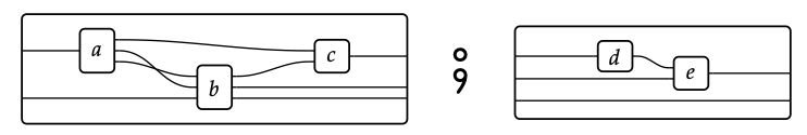
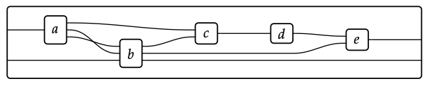
$Screen Shot 2021-02-09 at 6.52.53 PM.png$

El resultado es:

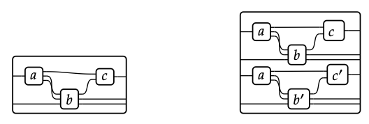
$Screen Shot 2021-02-09 at 6.53.23 PM.png$

Ejercicio 5.18

El producto monoidal de dos morfismos se dibuja apilando las gráficas de puertos correspondientes. Para este problema, simplemente apilamos la imagen de la izquierda encima de sí misma para obtener la imagen de la derecha:

$Screen Shot 2021-02-09 en 7.03.41 PM.png$

Ejercicio 5.20

Tenemos una relación R$\subseteq$ P × P que genera un preorden ≤$_{P}$ sobre P, tenemos un preorden arbitrario (Q, ≤$_{Q}$) y una función f: P → Q, no necesariamente monótona.

Supongamos que por cada x, y$\in$ P, si R (x, y) entonces f (x) ≤ f (y); queremos mostrar que f es monótona, es decir, que para cada x ≤$_{P}$ y tenemos f (x) ≤$_{Q}$ f (y). Por definición de P siendo el cierre reflexivo, transitivo de R, tenemos x ≤$_{P}$ y iff existe n$\in$$\mathbb{N}$ y x$_{0}$,..., x$_{n}$ en P con x$_{0}$ = x y x$_{n}$ = y y R (x$_{i}$, x$_{i + 1}$) por cada 0 ≤ i ≤ n − 1. (El caso n = 0 maneja la reflexividad.) Pero entonces por suposición, R (x$_{i}$, x$_{i + 1}$) implica f (x$_{i}$) ≤$_{Q}$ f (x$_{i + 1}$) para cada i. Por inducción en i mostramos que f (x$_{0}$) ≤$_{Q}$ f (x$_{i}$) para todos 0 ≤ i ≤ n, momento en el que estamos hechos.
Supongamos ahora que f es monótona, y tomar x, y$\in$ P para la que R (x, y) sostiene. Entonces x ≤$_{P}$ y porque ≤$_{P}$ es la relación de preorden más pequeña que contiene R. (Otra forma de ver esto con base en la descripción anterior es con n = 1, x$_{0}$ = x, y x$_{n}$ = y, lo que dijimos implica x ≤$_{P}$ y.) Dado que f es monótona, efectivamente tenemos f (x) ≤$_{Q}$ f (y).

Ejercicio 5.21

Supongamos que P, Q y R son como en el Ejercicio 5.20 y tenemos una función g: Q → P.

Si R (g (a), g (b)) se mantiene para todos a ≤$_{Q}$ b entonces g es monótona, porque R (x, y) implica x ≤$_{P}$ y.
Es posible que g: (Q, ≤$_{Q}$) → (P, ≤$_{P}$) sea monótono y sin embargo tenga algunos a, b$\in$ Q con a ≤$_{Q}$ b y (g (a), g (b))$\not \in$ R. En efecto, toma Q: = {1} para ser el preorden libre en un elemento, y toma P: = {1} con R = Ø. Entonces la función única g: Q → P es monótona (porque ≤$_{P}$ es reflexiva aunque R esté vacía), y aún así (g (1), g (1))$\not \in$ R.

Ejercicio 5.23

Sea G = (V, A, s, t) una gráfica, que G sea la categoría libre en G, y que C sea otra categoría, cuyo conjunto de morfismos se denota Mor (C).

1. Dar una función Mor (C) → Ob (C) significa que por cada elemento Mor (C) necesitamos dar exactamente un elemento de Ob (C). Entonces para dom tomamos cualquier q$\in$ Mor (C), lo vemos como un morfismo q: y → z, y lo enviamos a su dominio y. De manera similar para bacalao: ponemos bacalao (q) := z.

2. Supongamos primero que se nos da un functor F: G → C. En los objetos tenemos una función Ob (G) → Ob (C), y esto define f desde Ob (G) = V. Sobre los morfismos, primero tenga en cuenta que las flechas de la gráfica G son exactamente la longitud = 1 caminos en G, mientras que Mor (G) es el conjunto de todos los caminos en G, por lo que tenemos una inclusión A$\subseteq$ Mor (G). El functor F proporciona una función Mor (G) → Mor (C), que podemos restringir a A para obtener g: A → Mor (C). Todos los funtores satisfacen dom (F (r)) = F (dom (r)) y cod (F (r)) = F (cod (r)) para cualquier r: w → x. En particular cuando r$\in$ A es una flecha tenemos dom (r) = s (r) y cod (r) = t (r).

Así hemos encontrado (f, g) con las propiedades requeridas.

Supongamos segundo que se nos da un par de funciones (f, g) donde f: V → Ob (C) y g: A → Mor (C) tal que dom (g (a)) = f (s (a)) y cod (g ( a)) = f (t (a)) para todos $\in$a A. Definir F: G → C en objetos por f. Un morfismo arbitrario en G es un camino p: = (v$_{0}$, a$_{1}$, a$_{2}$,..., a$_{n}$) en G, donde v$_{0}$$\in$ V, a$_{i}$ $\in$A, v$_{0}$ = s (a$_{1}$), y t (a$_{i}$) = s (a$_{i + 1}$) para todos 1 ≤ i ≤ n − 1. Entonces (a$_{i}$) es un morfismo en C cuyo dominio es f (v$_{0}$) y los morfismos (a$_{i}$) y (a$_{i + 1}$) son componibles por cada 1 ≤ i ≤ n − 1. Luego tomamos F (p) := id$_{f(v0)}$; g (a$_{1}$); · · ·; g (a$_{n}$) para ser el compuesto. Es fácil comprobar que efectivamente se trata de un functor (conserva identidades y composiciones).

Tercero, queremos ver que las dos operaciones que acabamos de dar son mutuamente inversas. En los objetos esto es sencillo, y en los morfismos es sencillo ver que, dado (f, g), si los convertimos en un functor F: G → C y luego extraemos el nuevo par de funciones (f ′, g ′), entonces f = f ′y g = g'. Finalmente, dado un functor F: G → C, extraemos el par de funciones (f, g) como arriba y luego las convertimos en un nuevo functor F ′: G → C. Está claro que F y F ′ actúan igual sobre los objetos, entonces qué pasa con los morfismos. La fórmula dice que F ′ actúa igual sobre morfismos de longitud 1 en G (es decir, sobre los elementos de A). Pero un morfismo arbitrario en G no es más que un camino, es decir, una secuencia de flechas componibles, y así por funcionalidad, tanto F como F ′ deben actuar igual en caminos arbitrarios.

3. (Mor (C), Ob (C), dom, cod) es una gráfica; vamos a denotarla U (C)$\in$ Grph. Tenemos funtores Libre: Grph$\rightleftharpoons$ Cat: U, y Free se deja colindante a U.

Ejercicio 5.24

1. Los elementos del monoide libre en el conjunto {a} son:

a$^{0}$, a$^{1}$, a$^{2}$, a$^{3}$,..., a$^{2019}$,...

con multiplicación monoide ∗ dada por la suma habitual del número natural en los exponentes, a$^{i}$ ∗ a$^{j}$ = a$^{i + j}$.

2. Esto es isomórfico a$\mathbb{N}$, enviando un$^{i}$ $\mapsto$i.

3. Los elementos del monoide libre en el conjunto {a, b} son 'palabras en a y b', cada una de las cuales representaremos como una lista cuyas entradas son a o b. Aquí hay algunos:

[], [a], [b], [a, a], [a, b],..., [b, a, b, b, a, b, a, b, a, a, a],...

Ejercicio 5.28

Tenemos dos apoyos: el prop de las gráficas portuarias y el prop libre Free (G, s, t) donde

G: = {ρ$_{m, n}$: m → n | m, n$\in$$\mathbb{N}$}, s (ρ$_{m, n}$ := m, t (ρ$_{m, n}$ := n;

queremos demostrar que son el mismo utilero. Como categorías tienen el mismo conjunto de objetos (en ambos casos,

N), por lo que necesitamos demostrar que por cada m, n$\in$$\mathbb{N}$, tienen el mismo conjunto de morfismos (y que sus fórmulas de composición y fórmulas de producto monoidales coinciden).

Por Definición 5.25, un morfismo m → n en Libre (G) es un gráfico de puertos con etiqueta G, es decir, un par (γ, l), donde γ = (V, in, out, ι) es un gráfico de puerto (m, n) y l: V → G es una función, tal que las 'peculiaridades concuerdan'. ¿Qué significa esto? Recordemos que cada vértice v$\in$ V se dibuja como una caja con algunos puertos de la izquierda y algunos puertos de la derecha una arity y l (v)$\in$ G se supone que tienen la arity correcta; precisamente, s (l (v)) = in ( v) y t (l (v)) = out (v). Pero G fue elegido para que tenga exactamente un elemento con cualquier aridad dada, por lo que la función l solo tiene una opción, y así no aporta nada: no aumenta ni disminuye la libertad. Es decir, un morfismo en nuestro particular Libre (G) puede identificarse con una gráfica portuaria (m, n) γ, según se desee.

Nuevamente por definición Definición 5.25, la 'composición y la estructura monoidal son solo las de las gráficas de puertos PG (ver Eq. (5.17)); las etiquetas (las l) simplemente se llevan a lo largo. ' Entonces ya terminamos.

Ejercicio 5.32

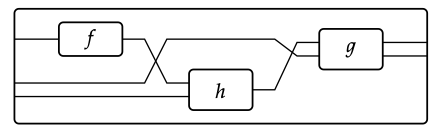
Aquí hay una imagen de (f + id$_{1}$ + id$_{1}$); (σ + id$_{1}$); (id$_{1}$ + h); σ; g, en el prop libre sobre generadores G = {f: 1 → 1, g: 2 → 2, h: 2 → 1}:

$Screen Shot 2021-02-09 a las 9.01.08 PM.png$

Ejercicio 5.35

El apuntalamiento libre sobre generadores (G, s, t), definido en la Definición 5.25, es para todos los efectos lo mismo que el prop presentado por (G, s, t, Ø), sin tener relaciones. La única “diferencia sutil” posible que podríamos tener que admitir es si alguien dijera que un conjunto S es “sutilmente diferente” de su cociente por la relación de equivalencia trivial. En este último, los elementos son los subconjuntos singleton de S. Entonces por ejemplo el cociente de S = {1, 2, 3} por la relación de equivalencia trivial es el conjunto ({1}, {2}, {3}). Es sutilmente diferente a S, pero los dos son naturalmente isomórficos, y categóricamente, la diferencia nunca hará la diferencia.

Ejercicio 5.41

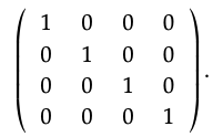
1. Si (R, 0, +, 1, ∗) es una plataforma, entonces la identidad multiplicativa 1$\in$ Mat$_{n}$ (R) es la matriz de identidad n -by- n habitual: 1's en la diagonal y 0's en todas partes (donde por '1' y '0', nos referimos a esos elementos de R). Entonces para n = 4 es:

$Screen Shot 2021-02-09 a las 9.18.44 PM.png$

2. Elegimos n = 2 y de ahí necesitamos encontrar dos elementos A, B$\in$ Mat$_{2}$ ($\mathbb{N}$) tal que A ∗ B$\neq$ B ∗ A.

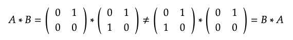
$Screen Shot 2021-02-09 a las 9.19.19 PM.png$

Se puede calcular a partir de la fórmula de multiplicación (recordada en el Ejemplo 5.40) dice (A ∗ B) (1, 1) = 0 ∗ 0 + 1 ∗ 1 = 1 y (B ∗ A) (1, 1) = 0 ∗ 0 + 0 ∗ 0 = 0, que no son iguales.

Ejercicio 5.43

Semánticamente, si aplicamos el gráfico de flujo a continuación a la señal de entrada (x, y)

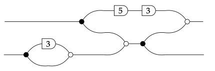
$Screen Shot 2021-02-09 a las 9.32.25 PM.png$

la señal de salida resultante es (16 x + 4 y, x + 4 y).

Ejercicio 5.51

El producto monoidal de A =$\begin{pmatrix} 3 & 3 & 1 \\ 2 & 0 & 4 \end{pmatrix}$ y B =$\begin{pmatrix} 2 & 5 & 6 & 1\end{pmatrix}$ es

A + B =$\begin{pmatrix} 3 & 3 &1 & 0 & 0 & 0 & 0 \\ 2 & 0 & 4 & 0 & 0 & 0 & 0 \\ 0 & 0 & 0 & 2 & 5 & 6 & 1 \end{pmatrix}$

Ejercicio 5.55

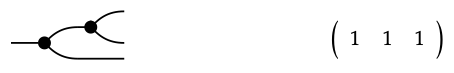
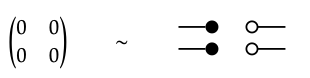
1. El gráfico de flujo de señal a la izquierda representa la matriz de la derecha:

$Screen Shot 2021-02-09 a las 9.39.38 PM.png$

2. El gráfico de flujo de señal a la izquierda representa la matriz de la derecha:

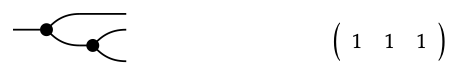
$Screen Shot 2021-02-09 a las 9.41.20 PM.png$

3. Ellos son iguales.

Ejercicio 5.58

1. $Screen Shot 2021-02-09 a las 9.46.12 PM.png$

2. $Screen Shot 2021-02-09 a las 9.46.55 PM.png$

3. $Screen Shot 2021-02-09 a las 9.49.57 PM.png$

Ejercicio 5.59

• Para la primera capa g$_{1}$, take the monoidal product of m copies of c$_{n}$,

g$_{1}$ := c$_{n}$ + · · · + c$_{n}$ : m → (m × n),

where c$_{n}$ is the signal flow diagram that makes n copies of a single input:

c$_{n}$ := ; (1+ ) ; (1 + 1+ ) ; ··· ; (1 + ··· + 1 + ) : 1 → n

• Next, define

g$_{2}$ := s$_{M(1,1)}$ + ··· + s$_{M(1,n)}$

+ s$_{M(2,1)}$ + · · · + s$_{M(2,n)}$

+ ···

+ s$_{M(m,1)}$ + · · · + s$_{M(m,n)}$ : (m × n) → (m × n),

where s$_{a}$ : 1 → 1 is the signal flow graph generator “scalar multiplication by a.” This layer amplifies each copy of the input signal by the relevant rig element.

The third layer rearranges wires. We will not write this down explicitly, but simply say it is the signal flow graph g$_{3}$ : m × n → m × n, that is the composite and monoidal product of swap and identity maps, such that the (i − 1)m + j th input is sent to the (j − 1)n + i th output, for all 1 ≤ i ≤ n and 1 ≤ j ≤ m.
Finally, the fourth layer is similar to the first, but instead adds the amplified input signals. We define

g$_{4}$ := a$_{m}$ + · · · + a$_{m}$ : (m × n) → n,

where a$_{m}$ is the signal flow graph that adds m inputs to produce a single output:

a$_{m}$ := (1 + ··· + 1 + ) ; ··· ; (1 + 1 + ) ; (1 + ) ; :m→1

Using Proposition 5.54, it is a straightforward but tedious calculation to show that g = g$_{1}$ ; g$_{2}$ ; g$_{3}$ ; g$_{4}$ : m → n has the property that S(g) = M

Exercise 5.62

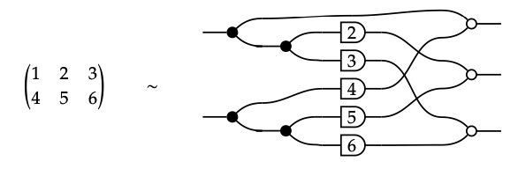
1. The matrices in Exercise 5.58 may also be drawn as the following signal flow graphs:

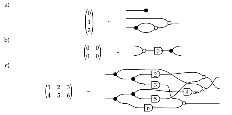
$Screen Shot 2021-02-09 at 10.00.56 PM.png$

2. Here are graphical proofs that there presentations we chose in our solution to Exercise 5.58 agree with those chosen in Part 1 above.

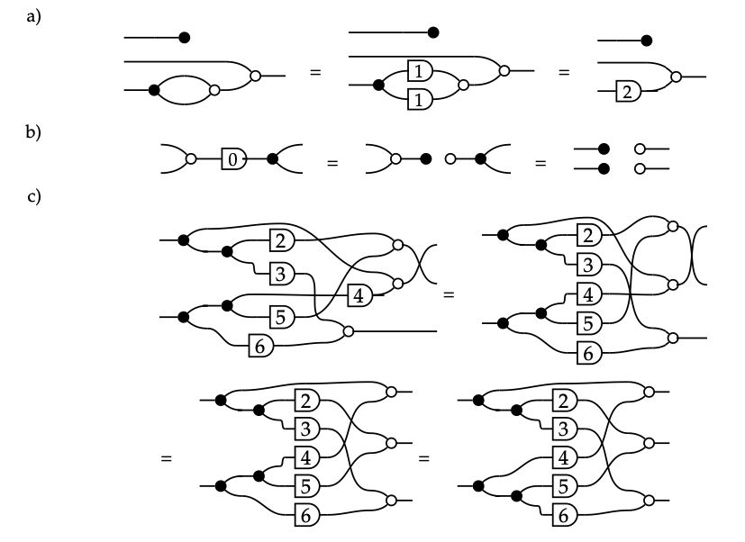
$Screen Shot 2021-02-09 at 10.42.50 PM.png$

Exercise 5.63

1. The signal flow graphs

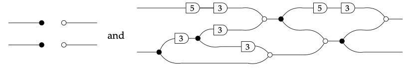
$Screen Shot 2021-02-09 at 10.44.47 PM.png$

cannot represent the same morphism because one has a path from a vertex on the left to one on the right, and the other does not. To prove this, observe that the only graphical equation in Theorem 5.60 that breaks a path from left to right is the equation

$Screen Shot 2021-02-09 at 10.45.12 PM.png$

So a 0 scalar must within a path from left to right before we could rewrite the diagram to break that path. No such 0 scalar can appear, however, because the diagram does not contain any, and the sum and product of any two nonzero natural numbers is always nonzero.

2. Replacing each of the 3s with 0 allows us to rewrite the diagram to

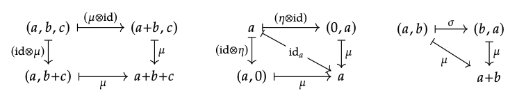
$Screen Shot 2021-02-09 at 10.45.43 PM.png$

Exercise 5.67

The three conditions of Definition 5.65 are

(a) (μ ⊗ id) ; μ = (id ⊗ μ) ; μ,

(b) (η ⊗ id) ; μ = id = (id ⊗ η) ; μ, and

where σ$_{M,M}$ is the swap map on M in C.
1. Suppose μ : $mathbb{R}$ × $mathbb{R}$ → $mathbb{R}$ is defined by μ(a, b) = a ∗ b and η $\in$ $mathbb{R}$ is defined to be η = 1. The conditions, written diagrammatically, say that starting in the upper left of each diagram below, the result in the lower right is the same regardless of which path you take:

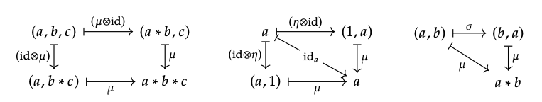
$Screen Shot 2021-02-09 at 10.53.17 PM.png$

and this is true for ($mathbb{R}$, *, 1).

2. The same reasoning works for ($mathbb{R}$, +, 0), shown below:

$Screen Shot 2021-02-09 at 10.54.30 PM.png$

Exercise 5.69

The functor U: Mat(R) → Set is given on objects by sending n to the set R$^{n}$, and on morphisms by matrix-vector multiplication. Here R$^{n}$ means the set of n-tuples or n-dimensional vectors in R. In particular, R$^{0}$ = {()} consists of a single vector of dimension 0.

1. U preserves the monoidal unit because 0 is the monoidal unit of any prop (Mat(R) is a prop), {1} is the monoidal unit of Set, and R$^{0}$ is canonically isomorphic to {1}. U also preserves the monoidal product because there is a canonical isomorphism R$^{m}$ × R$^{n}$ $\cong$ R$^{m + n}$.

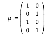
2. A monoid object in Mat(R) is a tuple (m, μ, η) where m $\in$ $\mathbb{N}$, μ : m + m → m, and η : 0 → m satisfy the properties μ(η, x) = x = μ(x, η) and μ(x, μ(y, z)) = μ(μ(x, y), z). Note that there is only one morphism 0 → m in Mat(R) for any m. It is not hard to show that for any m $\in$ N there is only one monoid structure. For example, when m = 2, μ must be the following matrix

$Screen Shot 2021-02-10 at 10.58.58 PM.png$

Anyway, for any monoid (m, μ, η), the morphism U(η): R$^{0}$ → R$^{m}$ is given by U(η)(1) := (0, . . . , 0), and the morphism U(μ): R$^{m}$ × R$^{m}$ → R$^{m}$ is given by

U(μ)((a$_{1}$, . . . , a$_{m}$), (b$_{1}$, . . . , b$_{m}$)) := (a$_{1}$ + b$_{1}$, . . . , a$_{m}$ + b$_{m}$).

These give R$^{m}$ the structure of a monoid.

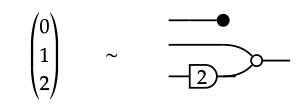
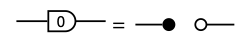
3. The triple (1, , o-) corresponds to the additive monoid structure on $\mathbb{R}$, e.g. with (5, 3) $\mapsto$ 8.

Exercise 5.77

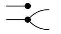
1. The behavior B() of the reversed addition icon : 1 →2 is the relation {(x, y, z) $\in$ R$^{3}$ | x = y + z}.

2. The behavior B() of the reversed addition icon : 1 →2 is the relation {(x, y, z) $\in$ R$^{3}$ | x = y + z}.

Exercise 5.80

If B $\subseteq$ R$^{m}$ ×R$^{n}$ andC $\subseteq$ R$^{p}$ ×R$^{q}$ are morphisms in Rel R, then take B + C $\subseteq$ R$^{m + p}$ ×R$^{n + q}$ to be the set

B + C := {(w, y, x, z) $\in$ R$^{m + p}$ × R$^{n + q}$ | (w, x) $\in$ B and (y, z) $\in$ C}.

Exercise 5.82

The behavior of g : m → n and h$^{op}$ : n → l are respectively

B(g) = {(x, z) $\in$ R$^{m}$ × R$^{n}$ | S(g)(x) = z}

B(h$^{op}$) = {(z, y) $\in$ R$^{n}$ × R$^{l}$ | z = S(h)(y)}

and by Eq. (5.78), the composite B(g ; (h$^{op}$)) = B(g) ; B(h$^{op}$) is:

{(x, y) | there exists z $\in$ R$^{n}$ such that S(g)(x) = z and z = S(h)(y)}.

Since S(g) and S(h) are functions, the above immediately reduces to the desired formula:

B(g ; (h$^{op}$)) = {(x, y) | S(g)(x) = S(h)(y)}.

Exercise 5.83

The behavior of g$^{op}$ : n → m and h : m → p are respectively

B(g$^{op}$) = {(y, x) $\in$ R$^{n}$ × R$^{m}$ | y = S(g)(x)}

B(h) = {(x, z) $\in$ R$^{m}$ × R$^{p}$ | S(h)(x) = z}

and by Eq. (5.78), the composite B(g$^{op}$) ; h) = B(g$^{op}$) ; B(h) is:

{(y, z) | there exists x $\in$ R$^{m}$ such that y = S(g)(x) and S(h)(x) = z}.

This immediately reduces to the desired formula:

B(g$^{op}$) ; h) = {(S(g)(x), S(h)(x)) | x $\in$ R$^{m}$ }.

Exercise 5.84

1. The behavior of the 0-reverse is the subset {y $\in$ R | y = 0}, and its n-fold tensor is similarly {y $\in$ R$^{n}$ | y = 0}.

Composing this relation with S(g) $\subseteq$ R$^{m}$ × R$^{n}$ gives {x $\in$ R$^{m}$ | S(g) = 0}, which is the kernel of S(g).

2. The behavior of the discard-inverse -o is the subset {x $\in$ R}, i.e. the largest subset of R, and similarly its m-fold tensor is R$^{n}$ $\subseteq$ R$^{n}$.

Composing this relation with S(g) $\subseteq$ R$^{m}$ × R$^{n}$ gives {y $\in$ R$^{n}$ | there exists x $\in$ R$^{m}$ such that S(g)(x) = y}, which is exactly the image of S(g).

3. For any g : m → n, we first claim that the behavior B(g) = {(x, y) | S(g)(x) = y} is linear, i.e. it is closed under addition and scalar multiplication. Indeed, S(g) is multiplication by a matrix, so if S(g)(x) = y then S(g)(rx) = ry and S(g)(x$_{1}$ + x$_{2}$) = S(g)(x$_{1}$) + S(g)(x$_{2}$).

Thus we con- clude that (x, y) $\in$ B(g) implies (rx, ry) $\in$ B(g), so it’s closed under scalar multiplication, and (x$_{1}$, y$_{1}$), (x$_{2}$, y$_{2}$) $\in$ B(g) implies (x$_{1}$ + x$_{2}$, y$_{1}$ + y$_{2}$) $\in$ B(g) so it’s closed under addition. Similarly, the behavior B(g$^{op}$) is also linear; the proof is similar.

Finally, we need to show that the composite of any two linear relations is linear. Suppose that B $\subseteq$ R$^{m}$ × R$^{n}$ and C $\subseteq$ R$^{n}$ × R$^{p}$ are linear. Take (x$_{1}$, z$_{1}$), (x$_{2}$, z$_{2}$) $\in$ B ; C and take r $\in$ R.

By definition, there exist y$_{1}$, y$_{2}$ $\in$ R$^{n}$ such that (x$_{1}$, y$_{1}$), (x$_{2}$, y$_{2}$) $\in$ B and (y$_{1}$, z$_{1}$), (y$_{2}$, z$_{2}$) $\in$ C. Since B and C are linear, (rx$_{1}$, ry$_{1}$) $\in$ B and (ry$_{1}$, rz$_{1}$) $\in$ C, and also (x$_{1}$ + x$_{2}$, y$_{1}$ + y$_{2}$) $\in$ B and (y$_{1}$ + y$_{2}$, z$_{1}$ + z$_{2}$) $\in$ C.

Hence (rx$_{1}$, rz$_{1}$) $\in$ (B ; C) and (x$_{1}$ + x$_{2}$, z$_{1}$ + z$_{2}$) $\in$ (B ; C), as desired.

Exercise 5.85

Suppose that B $\subseteq$ R$^{m}$ × R$^{n}$ and C $\subseteq$ R$^{n}$ × R$^{p}$ are linear. Their composite is the relation (B ; C) $\subseteq$ R$^{m}$ × R$^{p}$ consisting of all (x, z) for which there exists y $\in$ R$^{n}$ with (x, y) $\in$ B and (y, z) $\in$ C. We want to show that the set (B ; C) is linear, i.e. closed under scalar multiplication and addition.
For scalar multiplication, take an (x, z) $\in$ (B ; C) and any r $\in$ R.

Since B is linear, we have (r ∗ x, r ∗ y) $\in$ B and since C is linear we have (r ∗ y, r ∗ z) $\in$ C,so then (r ∗ x, r ∗ z) $\in$ (B ; C). For addition, if we also have (x′, z′) $\in$ (B ; C) then there is some y′ $\in$ Rn with(x′,y′) $\in$ B and(y′,z′) $\in$ C, so since B and C are linear we have (x + x′, y + y′) $\in$ B and (y + y′, z + z′) $\in$ C, hence (x + x′, z + z′) $\in$ (B ; C).