
4.3.4: Resolver Sistemas de Ecuaciones
- Page ID
- 118694

Lección
Resolvamos sistemas de ecuaciones.
Ejercicio\(\PageIndex{1}\): True or False: Two Lines
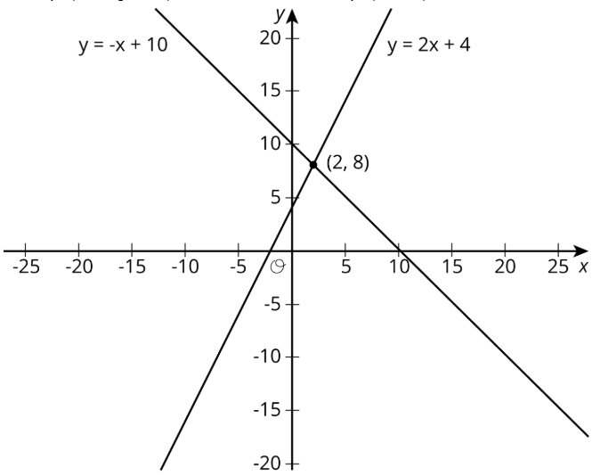
Usa las líneas para decidir si cada declaración es verdadera o falsa. Esté preparado para explicar su razonamiento usando las líneas.
- Una solución a\(8=-x+10\) es 2.
- Una solución a\(2=2x+4\) es 8.
- Una solución a\(-x+10=2x+4\) es 8.
- Una solución a\(-x+10=2x+4\) es 2.
- No hay valores de\(x\) y\(y\) que hacen\(y=-x+10\) y\(y=2x+4\) verdad al mismo tiempo.
Ejercicio\(\PageIndex{2}\): Matching Graphs to Systems
Aquí hay tres sistemas de ecuaciones gráficas en un plano de coordenadas:
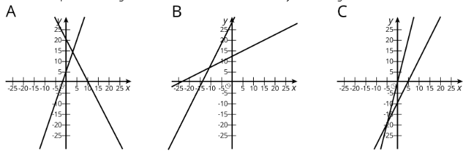
- Haga coincidir cada figura con uno de los sistemas de ecuaciones que se muestran aquí.
- \(\left\{\begin{array}{l}{y=3x+5}\\{y=-2x+20}\end{array}\right.\)
- \(\left\{\begin{array}{l}{y=2x-10}\\{y=4x-1}\end{array}\right.\)
- \(\left\{\begin{array}{l}{y=0.5x+12}\\{y=2x+27}\end{array}\right.\)
- Encuentre la solución para cada sistema y luego verifique que su solución sea razonable en la gráfica.
- Observe que los deslizadores establecen los valores del coeficiente y el término constante en cada ecuación.
- Cambiar los deslizadores a los valores del coeficiente y el término constante en el siguiente par de ecuaciones.
- Haga clic en el lugar donde se cruzan las líneas y debería aparecer un punto etiquetado.
Ejercicio\(\PageIndex{3}\): Different Types of Systems
Tu profesor te dará una página con 6 sistemas de ecuaciones.
- Grafica cada sistema de ecuaciones escribiendo cada par de ecuaciones en el applet, una a la vez.
- Describir cómo se ve la gráfica de un sistema de ecuaciones cuando tiene.
- 1 solución
- 0 soluciones
- infinitamente muchas soluciones
Usa el applet para confirmar tu respuesta a la pregunta 2.
¿Estás listo para más?
Las gráficas de las ecuaciones\(Ax+By=15\) y se\(Ax-By=9\) cruzan en\((2,1)\). Encontrar\(A\) y\(B\). Muestra o explica tu razonamiento.
Resumen
A veces es más fácil resolver un sistema de ecuaciones sin tener que graficar las ecuaciones y buscar un punto de intersección. En general, siempre que estemos resolviendo un sistema de ecuaciones escritas como
\[\left\{\begin{array}{l}{y=\text{[some stuff]}}\\{y=\text{[some other stuff]}}\end{array}\right.\nonumber\]
sabemos que estamos buscando un par de valores\((x,y)\) que hagan verdaderas ambas ecuaciones. En particular, sabemos que el valor para\(y\) será el mismo en ambas ecuaciones. Eso significa que
\[\text{[some stuff]}=\text{[some other stuff]}\nonumber\]
Por ejemplo, mira este sistema de ecuaciones:
\[\left\{\begin{array}{l}{y=2x+6}\\{y=-3x-4}\end{array}\right.\nonumber\]
Dado que el\(y\) valor de la solución es el mismo en ambas ecuaciones, entonces sabemos\(2x+6=-3x-4\)
Podemos resolver esta ecuación para\(x\):
\[\begin{aligned} 2x+6&=-3x-4 \\ 5x+6&=-4 &\text{add 3x to each side} \\ 5x&=-10 &\text{subtract 6 from each side} \\ x&=-2 &\text{divide each side by 5}\end{aligned}\nonumber\]
Pero esto es sólo la mitad de lo que estamos buscando: conocemos el valor para\(x\), pero necesitamos el valor correspondiente para\(y\). Dado que ambas ecuaciones tienen el mismo\(y\) valor, podemos usar cualquiera de las dos ecuaciones para encontrar el\(y\) -value:
\(y=2(-2)+6\)
O
\(y=-3(-2)-4\)
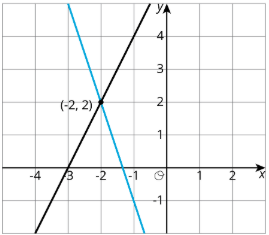
En ambos casos, nos encontramos con eso\(y=2\). Entonces la solución al sistema es\((-2,2)\). Podemos verificar esto graficando ambas ecuaciones en el plano de coordenadas.
En general, un sistema de ecuaciones lineales puede tener:
- Sin soluciones. En este caso, las líneas que corresponden a cada ecuación nunca se cruzan.
- Exactamente una solución. Las líneas que corresponden a cada ecuación se cruzan en exactamente un punto.
- Un número infinito de soluciones. ¡Las gráficas de las dos ecuaciones son la misma línea!
Entradas en el glosario
Definición: Sistema de ecuaciones
Un sistema de ecuaciones es un conjunto de dos o más ecuaciones. Cada ecuación contiene dos o más variables. Queremos encontrar valores para las variables que hagan verdaderas todas las ecuaciones.
Estas ecuaciones conforman un sistema de ecuaciones:
\[\left\{\begin{array}{l}{x+y=-2}\\{x-y=12}\end{array}\right.\nonumber\]
La solución a este sistema es\(x=5\) y\(y=-7\) porque cuando estos valores son sustituidos por\(x\) y\(y\), cada ecuación es verdadera:\(5+(-7)=-2\) y\(5-(-7)=12\).
Practica
Ejercicio\(\PageIndex{4}\)
1. Escribe ecuaciones para las líneas mostradas.
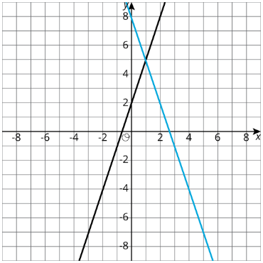
2. Describir cómo encontrar la solución al sistema correspondiente mirando la gráfica.
3. Describir cómo encontrar la solución al sistema correspondiente mediante el uso de las ecuaciones.
Ejercicio\(\PageIndex{5}\)
La solución a un sistema de ecuaciones es\((5,-19)\). Elija dos ecuaciones que podrían formar el sistema.
- \(y=-3x-6\)
- \(y=2x-23\)
- \(y=-7x+16\)
- \(y=x-17\)
- \(y=-2x-9\)
Ejercicio\(\PageIndex{6}\)
Resuelve el sistema de ecuaciones:
\[\left\{\begin{array}{l}{y=4x-3}\\{y=-2x+9}\end{array}\right.\nonumber\]
Ejercicio\(\PageIndex{7}\)
Resuelve el sistema de ecuaciones:
\[\left\{\begin{array}{l}{y=\frac{5}{4}x-2}\\{y=-\frac{1}{4}x+19}\end{array}\right.\nonumber\]
Ejercicio\(\PageIndex{8}\)
Aquí hay una ecuación:\(\frac{15(x-3)}{5}=3(2x-3)\)
- Resuelve la ecuación usando primero la propiedad distributiva.
- Resuelve la ecuación sin usar la propiedad distributiva.
- Consulta tu solución.
(De la Unidad 4.2.5)