
20.2: Ecuaciones que involucran funciones trigonométricas
- Page ID
- 117661

El apartado anterior mostró cómo resolver las ecuaciones trigonométricas básicas
\[\sin(x)=c, \quad \cos(x)=c, \quad \text{ and }\quad \tan(x)=c \nonumber \]
Los siguientes ejemplos se pueden reducir a estas ecuaciones básicas.
Resolver para\(x\).
- \(2\sin(x)-1=0\)
- \(\sec(x)=-\sqrt{2}\)
- \(7\cot(x)+3=0\)
Solución
- Resolviendo para\(\sin(x)\), obtenemos
\[2\sin(x)-1=0 \stackrel{(+1)}\implies 2\sin(x)=1 \stackrel{(\div 2)}\implies \sin(x)=\dfrac{1}{2} \nonumber \]
Una solución de\(\sin(x)=\dfrac 1 2\) es\(\sin^{-1}\left(\dfrac 1 2\right)=\dfrac {\pi}{6}\). La solución general es
\[x=(-1)^n\cdot \dfrac{\pi}{6}+n\pi, \quad \text{ where } n=0,\pm1,\pm2, \dots \nonumber \]
- Recordemos eso\(\sec(x)=\dfrac{1}{\cos(x)}\). Por lo tanto,
\[\sec(x)=-\sqrt{2} \implies \dfrac{1}{\cos(x)}=-\sqrt{2} \quad\stackrel{(\text{reciprocal})} \implies\quad \cos(x)=-\dfrac{1}{\sqrt{2}}=-\dfrac{\sqrt{2}}{2} \nonumber \]
Una solución especial de\(\cos(x)=-\dfrac{\sqrt{2}}{2}\) es
\[\cos^{-1}\left(-\dfrac{\sqrt{2}}{2}\right)=\pi-\cos^{-1}\left(\dfrac{\sqrt{2}}{2}\right)=\pi-\dfrac{\pi}{4}=\dfrac{4\pi-\pi}{4}=\dfrac{3\pi}{4} \nonumber \]
La solución general es
\[x=\pm\dfrac{3\pi}{4}+2n\pi, \quad \text{ where } n=0,\pm1,\pm2, \dots \nonumber \]
- Recordemos eso\(\cot(x)=\dfrac 1 {\tan(x)}\). Entonces
\[\begin{aligned} 7\cot(x)+3=0 &\stackrel{(-3)}\implies & 7\cot(x)=-3 \stackrel{(\div 7)}\implies \cot(x)=-\dfrac{3}{7} \\ &\implies & \dfrac 1 {\tan(x)}=-\dfrac{3}{7} \quad \stackrel{(\text{reciprocal})} \implies\quad \tan(x)=-\dfrac{7}{3} \end{aligned} \nonumber \]
La solución es
\[x=\tan^{-1}\left(-\dfrac{7}{3}\right)+n\pi \approx -1.166+n\pi, \quad \text{ where } n=0,\pm1,\pm2,\dots \nonumber \]
Para algunos de los problemas más avanzados puede ser útil sustituir\(u\) primero una expresión trigonométrica, luego resolver y finalmente aplicar las reglas de la sección anterior para resolver la variable deseada.\(u\) Este método se utiliza en el siguiente ejemplo.
Resolver para\(x\).
- \(\tan^2(x)+2\tan(x)+1=0\)
- \(2\cos^2(x)-1=0\)
Solución
- Sustituyendo\(u=\tan(x)\), tenemos que resolver la ecuación
\[u^2+2u+1=0 \stackrel{(\text{factor})}\implies (u+1)(u+1)=0 \implies u+1=0 \stackrel{(-1)}\implies u=-1 \nonumber \]
Resustituyendo\(u=\tan(x)\), tenemos que resolver\(\tan(x)=-1\). Usando el hecho de que\(\tan^{-1}(-1)=-\tan^{-1}(1)=-\dfrac{\pi}{4}\), tenemos la solución general
\[x=-\dfrac{\pi}{4}+n\pi, \quad \text{ where } n=0,\pm1,\pm2, \dots \nonumber \]
- Nosotros sustituimos\(u=\cos(x)\), entonces tenemos
\[\begin{aligned} 2u^2-1=0 & \stackrel{(+1)}\implies & 2u^2=1 \quad \stackrel{(\div 2)}\implies \quad u^2=\dfrac 1 2 \\ & \implies & u=\pm\sqrt{\dfrac{1}{2}}=\pm\dfrac{1}{\sqrt{2}}=\pm\dfrac{\sqrt{2}}{2} \\ & \implies & u=+\dfrac{\sqrt{2}}{2} \quad\text{ or }\quad u=-\dfrac{\sqrt{2}}{2}\end{aligned} \nonumber \]
Para cada uno de los dos casos necesitamos resolver la ecuación correspondiente después de la sustitución\(u=\cos(x)\).
\ [\ begin {alineado}
\ cos (x) &=\ dfrac {\ sqrt {2}} {2}\
\ texto {con}\ cos ^ {-1}\ izquierda (\ dfrac {\ sqrt {2}} {2}\ derecha) &=\ dfrac {\ pi} {4}\\
\ Longrightarrow x&=\ pm\ dfrac {pi} {4} +2 n\ pi &\ texto {donde} n=0,\ pm 1,\ pm 2,\ lpuntos
\ final {alineado}\ nonumber\]
\ [\ begin {alineado}
\ cos (x) &=-\ dfrac {\ sqrt {2}} {2}\\
&\ texto {con}\ begin {alineado}
\ cos ^ {-1}\ izquierda (-\ dfrac {\ sqrt {2}} {2}\ derecha) &=\ pi-\ cos ^ {-1}\ izquierda (\ dfrac {\ sqrt {\ sqrt {2}} {2}\ derecha)\\
&=\ pi-\ dfrac {\ pi} {4} =\ dfrac {3\ pi} {4}
\ end { alineado}\\
\ Longrightarrow x&=\ pm\ dfrac {3\ pi} {4} +2 n\ pi\\
&\ texto {donde} n=0,\ pm 1,\ pm 2,\ lpuntos
\ final {alineado}\ nonumber\]
Así, la solución general es
\[x=\pm\dfrac{\pi}{4}+2n\pi,\quad \text{ or } \quad x=\pm\dfrac{3\pi}{4}+2n\pi, \quad \text{ where } n=0,\pm1, \pm2,\dots \nonumber \]
Resuelve la ecuación con la calculadora. Aproximar la solución a la milésima más cercana.
- \(2\sin(x)=4\cos(x)+3\)
- \(5\cos(2x)=\tan(x)\)
Solución
- Reescribimos la ecuación como\(2\sin(x)-4\cos(x)-3=0\), y usamos la calculadora para encontrar la gráfica de la función\(f(x)=2\sin(x)-4\cos(x)-3\). Los ceros de la función\(f\) son las soluciones de la ecuación inicial. A continuación se muestra la gráfica que obtenemos.
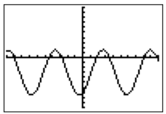
El gráfico indica que la función\(f(x)=2\sin(x)-4\cos(x)-3\) es periódica. Esto se puede confirmar observando que ambos\(\sin(x)\) y\(\cos(x)\) son periódicos con periodo\(2\pi\), y por lo tanto también\(f(x)\).
\[f(x+2\pi)= 2\sin(x+2\pi)-4\cos(x+2\pi)-3=2\sin(x)-4\cos(x)-3=f(x) \nonumber \]
La solución de se\(f(x)=0\) puede obtener encontrando los “ceros”, es decir, presionando\(\boxed{\text{2nd}} \boxed{\text{trace}} \boxed{\text{2}}\), luego eligiendo un límite izquierdo y derecho, y haciendo una suposición para el cero. Repetir este procedimiento da las siguientes dos soluciones aproximadas dentro de un periodo.
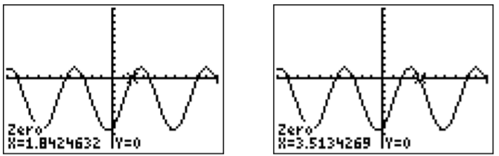
La solución general es así
\[x\approx1.842+2n\pi \quad \text{ or } \quad x\approx3.513+2n\pi, \quad \text{ where } n=0,\pm1,\pm2,\dots \nonumber \]
- Reescribimos la ecuación como\(5\cos(2x)-\tan(x)=0\) y graficamos la función\(f(x)=5\cos(2x)-\tan(x)\) en la ventana estándar.
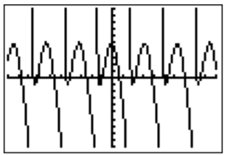
Para obtener una mejor visión de la función nos acercamos a una ventana más apropiada.
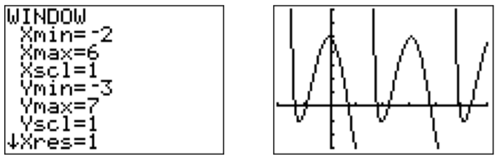
Obsérvese nuevamente que la función\(f\) es periódica. El periodo de\(\cos(2x)\) es\(\dfrac{2\pi}{2}=\pi\) (ver definición [def:Amplitude-periodo-fase] en la página), y el periodo de\(\tan(x)\) es también\(\pi\) (ver ecuación [equ:tan-period] en la página). Así, también\(f\) es periódico con periodo\(\pi\). Las soluciones en un periodo se aproximan encontrando los ceros con la calculadora.
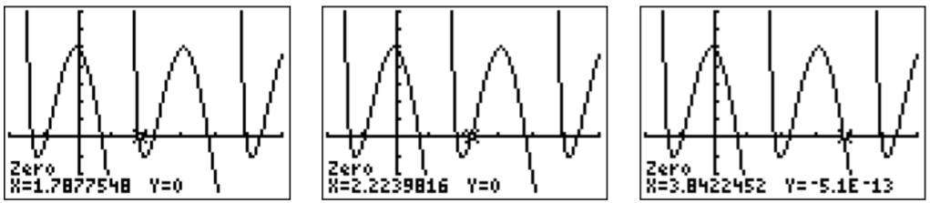
La solución general viene dada por cualquiera de estos números, con posiblemente un cambio adicional por cualquier múltiplo de\(\pi\).
\ [\ comenzar {alineado}
x\ aprox 1.788+n\ pi\ quad\ texto {o}\ quad x\ aprox 2.224+n\ pi\ quad\ texto {o}\ quad x\ approx 3.842+n\ pi\ quad\ texto {donde} n=0,\ pm 1,\ pm 2,\ pm 3,\ ldots\ final {alineado}\ nonumber\]