1.21: Resolviendo las ecuaciones seculares

Formulación matricial de un conjunto de ecuaciones lineales

Como ya hemos visto, cualquier conjunto de ecuaciones lineales puede ser reescrito como una ecuación matricial\(A\textbf{x}\) = \(\textbf{b}\). Linear equations are classified as simultaneous linear equations or homogeneous linear equations, depending on whether the vector \(\textbf{b}\) on the RHS of the equation is non-zero or zero.

Para un conjunto de ecuaciones lineales simultáneas (distintas de cero\(\textbf{b}\)) it is fairly apparent that if a unique solution exists, it can be found by multiplying both sides by the inverse matrix \(A^{-1}\) (since \(A^{-1}A\) on the left hand side is equal to the identity matrix, which has no effect on the vector \(\textbf{x}\))

\[\begin{array}{rcl} A\textbf{x} & = & \textbf{b} \\ A^{-1}A\textbf{x} & = & A^{-1}\textbf{b} \\ \textbf{x} & = & A^{-1}\textbf{b} \end{array} \label{21.1}\]

En la práctica, existen métodos matriciales más fáciles para resolver ecuaciones simultáneas que encontrar la matriz inversa, pero estos no necesitan preocuparnos aquí. En la Sección 8.4, descubrimos que para que una matriz tenga una inversa, debe tener un determinante distinto de cero. Desde\(A^{-1}\) must exist in order for a set of simultaneous linear equations to have a solution, this means that the determinant of the matrix \(A\) must be non-zero for the equations to be solvable.

Lo contrario es cierto para ecuaciones lineales homogéneas. En este caso el conjunto de ecuaciones sólo tiene una solución si el determinante de\(A\) is equal to zero. The secular equations we want to solve are homogeneous equations, and we will use this property of the determinant to determine the molecular orbital energies. An important property of homogeneous equations is that if a vector \(\textbf{x}\) is a solution, so is any multiple of \(\textbf{x}\), meaning that the solutions (the molecular orbitals) can be normalized without causing any problems.

Resolviendo las energías orbitales y los coeficientes de expansión

Recordemos las ecuaciones seculares para\(A_1\) orbitals of \(NH_3\) derived in the previous section

\[\begin{array}{rcl} c_1(H_{11} - ES_{11}) + c_2(H_{12} - ES_{12}) & = & 0 \\ c_1(H_{12} - ES_{12}) + c_2(H_{22} - ES_{22}) & = & 0 \end{array} \label{21.2}\]

donde\(c_1\) and \(c_2\) are the coefficients in the linear combination of the SALCs \(\phi_1\) =\(s_N\) and \(\phi_2\) =\(\dfrac{1}{\sqrt{3}}(s_1 + s_2 + s_3)\) utilizado para construir el orbital molecular. Escribir este conjunto de ecuaciones lineales homogéneas en forma de matriz da

\[\begin{pmatrix} H_{11} - ES_{11} & H_{12} - ES_{12} \\ H_{12} - ES_{12} & H_{22} - ES_{22} \end{pmatrix} \begin{pmatrix} c_1 \\ c_2 \end{pmatrix} = \begin{pmatrix} 0 \\ 0 \end{pmatrix} \label{21.3}\]

Para que las ecuaciones tengan una solución, el determinante de la matriz debe ser igual a cero. Escribir el determinante nos dará una ecuación polinómica en\(E\) that we can solve to obtain the orbital energies in terms of the Hamiltonian matrix elements \(H_{ij}\) and overlap integrals \(S_{ij}\). The number of energies obtained by ‘solving the secular determinant’ in this way is equal to the order of the matrix, in this case two.

El determinante secular para la Ecuación\(\ref{21.3}\) is (noting that \(S_{11}\) = \(S_{22} = 1\) since the SALCs are normalized)

\[(H_{11} - E)(H_{22} - E) - (H_{12} - ES_{12})^2 = 0 \label{21.4}\]

Ampliar y recopilar términos en\(E\) gives

\[E^2(1-S_{12}^2) + E(2H_{12}S_{12} - H_{11} - H_{22}) + (H_{11}H_{22} - H_{12}^2) = 0 \label{21.5}\]

que se puede resolver usando la fórmula cuadrática para dar las energías de los dos orbitales moleculares.

\[E_\pm = \dfrac{-(2H_{12}S_{12} - H_{11} - H_{22}) \pm \sqrt{(2H_{12}S_{12} - H_{11} - H_{22})^2 - 4(1-S_{12}^2)(H_{11}H_{22} - H_{12}^2)}}{2(1-S_{12}^2)} \label{21.6}\]

Para obtener valores numéricos para las energías, necesitamos evaluar las integrales\(H_{11}\), \(H_{22}\), \(H_{12}\), and \(S_{12}\). This would be quite a challenge to do analytically, but luckily there are a number of computer programs that can be used to calculate the integrals. One such program gives the following values.

\[\begin{array}{rcl} H_{11} & = & -26.0000 \: eV \\ H_{22} & = & -22.2216 \: eV \\ H_{12} & = & -29.7670 \: eV \\ S_{12} & = & \: 0.8167 \: eV \end{array} \label{21.7}\]

Cuando sustituimos estos en nuestra ecuación por los niveles de energía, obtenemos:

\[\begin{array}{rcl} E_+ & = & \: 29.8336 \: eV \\ E_- & = & -31.0063 \: eV \end{array} \label{21.8}\]

Ahora tenemos las energías orbitales y el siguiente paso es encontrar los coeficientes orbitales. Los coeficientes para una órbita de energía\(E\) are found by substituting the energy into the secular equations and solving for the coefficients \(c_i\). Since the two secular equations are not linearly independent (i.e. they are effectively only one equation), when we solve them to find the coefficients what we will end up with is the relative values of the coefficients. This is true in general: in a system with \(N\) coefficients, solving the secular equations will allow all \(N\) of the coefficients \(c_i\) to be obtained in terms of, say, \(c_1\). The absolute values of the coefficients are found by normalizing the wavefunction.

Desde las ecuaciones seculares para los orbitales de la energía\(E_+\) and \(E_-\) are not linearly independent, we can choose to solve either one of them to find the orbital coefficients. We will choose the first.

\[(H_{11} - E_{\pm})c_1 + (H_{12} - E_{\pm}S_{12})c_2 = 0 \label{21.9}\]

Para el orbital con energía\(E_-\) = -31.0063 eV, substituting numerical values into this equation gives

\[\begin{array}{rcl} 5.0063 c_1 - 4.4442 c_2 & = & 0 \\ c_2 & = & 1.1265 c_1 \end{array} \label{21.10}\]

El orbital molecular es, por lo tanto

\[\Psi = c_1(\phi_1 + 1.1265\phi_2) \label{21.11}\]

Normalizar para encontrar la constante\(c_1\) (by requiring \(\label\Psi|\Psi \rangle\) = 1) da

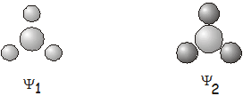
\[\begin{array}{rcll} \Psi_1 & = & 0.4933\phi_1 + 0.5557\phi_2 & \\ & = & 0.4933s_N + 0.3208(s_1 + s_2 + s_3) & (\text{substituting the SALCs for} \: \phi_1 \: \text{and} \: \phi_2) \end{array} \label{21.12}\]

Para el segundo orbital, con energía\(E_+\) = 29.8336 eV, the secular equation is

\[\begin{array}{rcl} -55.8336c_1 - 54.1321c_2 & = & 0 \\ c_2 & = & -1.0314c_1 \end{array} \label{21.13}\]

dando

\[\begin{array}{rcll} \Psi_2 & = & c_1(\phi_1 - 1.0314\phi_2) & \\ & = & 1.6242\phi_1 - 1.6752\phi_2 & \text{(after normalization)} \\ & = & 1.6242s_N -0.9672(s_1 + s_2 + s_3) \end{array} \label{21.14}\]

Estos dos\(A_1\) molecular orbitals \(\Psi_1\) y\(\Psi_2\) , uno de unión y otro antiadherentes, se muestran a continuación.

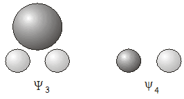
Las dos SALC restantes derivadas de la\(s\) orbitals of \(NH_3\):

\[\phi_3 = \dfrac{1}{\sqrt{6}}\begin{pmatrix} 2s_1 - s_2 - s_3 \end{pmatrix}\]

y

\[\phi_4 = \dfrac{1}{\sqrt{2}} \begin{pmatrix} s_2 - s_3 \end{pmatrix}\]

formar un par ortogonal de orbitales moleculares de\(E\) symmetry. We can show this by solving the secular determinant to find the orbital energies. The secular equations in this case are:

\[\begin{array}{rcl} c_1(H_{33} - ES_{33}) + c_2(H_{34} -ES_{34}) & = & 0 \\ c_1(H_{34} -ES_{34}) + c_2(H_{44} - ES_{44}) & = & 0 \end{array} \label{21.15}\]

Resolviendo el determinante secular da

\[E_\pm = \dfrac{-(2H_{34}S_{34} - H_{33} - H_{44}) \pm \sqrt{(2H_{34}S_{34} - H_{33} - H_{44})^2 - 4(1-S_{34}^2)(H_{33}H_{44} - H_{34}^2)}}{2(1-S_{34}^2)} \label{21.16}\]

Las integrales requeridas son

\[\begin{array}{rcl} H_{33} & = & -9.2892 \: eV \\ H_{44} & = & -9.2892 \: eV \\ H_{34} & = & 0 \\ S_{34} & = & 0 \end{array} \label{21.17}\]

Utilizando el hecho de que\(H_{34}\) = \(S_{34} = 0\), the expression for the energies reduces to

\[E_\pm = \dfrac{(H_{33} + H_{44}) \pm (H_{33} - H_{44})}{2} \label{21.18}\]

dando\(E_+\) = \(H_{33}\) = -9.2892 eV and \(E_-\) = \(H_{44}\) = -9.2892 eV. Each SALC therefore forms a molecular orbital by itself, and the two orbitals have the same energy; the two SALCs form an orthogonal pair of degenerate orbitals. These two molecular orbitals of \(E\) symmetry are shown below.