1.23: Un ejemplo de unión más complicado

Como otro ejemplo, utilizaremos la teoría de grupos para construir los orbitales moleculares de\(H_2O\) (point group \(C_{2v}\)) using a basis set consisting of all the valence orbitals. The valence orbitals are a \(1s\) orbital on each hydrogen, which we will label \(s_H\) and \(s_H'\), and a \(2s\) and three \(2p\) orbitals on the oxygen, which we will label \(s_O\), \(p_x\), \(p_y\), \(p_z\) giving a complete basis \(\begin{pmatrix} s_H, s_H', s_O, p_x, p_y, p_z \end{pmatrix}\).

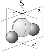
Lo primero que hay que hacer es determinar cómo cada orbital se transforma bajo las operaciones de simetría del\(C_{2v}\) point group (\(E\), \(C_2\), \(\sigma_v\) y\(\sigma_v'\) ), construir una representación matricial y determinar los caracteres de cada operación. A continuación se muestran las operaciones de simetría y el sistema de ejes que utilizaremos.

Los orbitales se transforman de la siguiente manera

\[\begin{array}{lrcl} E & \begin{pmatrix} s_H, s_H', s_O, p_x, p_y, p_z \end{pmatrix} & \rightarrow & \begin{pmatrix} s_H, s_H', s_O, p_x, p_y, p_z \end{pmatrix} \\ C_2 & \begin{pmatrix} s_H, s_H', s_O, p_x, p_y, p_z \end{pmatrix} & \rightarrow & \begin{pmatrix} s_H', s_H, s_O, -p_x, -p_y, p_z \end{pmatrix} \\ \sigma_v(xz) & \begin{pmatrix} s_H, s_H', s_O, p_x, p_y, p_z \end{pmatrix} & \rightarrow & \begin{pmatrix} s_H, s_H', s_O, p_x, -p_y, p_z \end{pmatrix} \\ \sigma_v'(yz) & \begin{pmatrix} s_H, s_H', s_O, p_x, p_y, p_z \end{pmatrix} & \rightarrow & \begin{pmatrix} s_H', s_H, s_O, -p_x, p_y, p_z \end{pmatrix} \end{array} \label{23.1}\]

Un breve aparte en la construcción de representantes de matriz

Después de un poco de práctica, probablemente podrás escribir representantes matriciales de inmediato con solo observar el efecto de las operaciones de simetría sobre la base. Sin embargo, si estás luchando un poco el siguiente procedimiento podría ayudar.

Recuerde que los representantes de la matriz son solo las matrices por las que tendríamos que multiplicar el lado izquierdo de las ecuaciones anteriores para dar el lado derecho. En la mayoría de los casos son muy fáciles de ejercitar. Probablemente la forma más sencilla de pensarlo es que cada columna de la matriz muestra dónde termina una de las funciones básicas originales. Por ejemplo, la primera columna transforma la función base\(s_H\) to its new position. The first column of the matrix can be found by taking the result on the right hand side of the above expressions, replacing every function that isn’t \(s_H\) with a zero, putting the coefficient of \(s_H\) (\(1\) or \(-1\) in this example) in the position at which it occurs, and taking the transpose to give a column vector.

Rotación

Considerar al representante para el\(C_2\) operation. The original basis \(\begin{pmatrix} s_H, s_H', s_O, p_x, p_y, p_z \end{pmatrix}\) transforms into \(\begin{pmatrix} s_H', s_H, s_O, -p_x, -p_y, p_z \end{pmatrix}\). Por lo tanto, la primera columna de la matriz se transforma\(s_H\) into \(s_H'\). Taking the result and replacing all the other functions with zeroes gives \(\begin{pmatrix} 0, s_H, 0, 0, 0, 0 \end{pmatrix}\). The coefficient of \(s_H\) is \(1\), so the first column of the \(C_2\) matrix representative is

\[\begin{pmatrix} 0 \\ 1 \\ 0 \\ 0 \\ 0 \\ 0 \end{pmatrix} \label{23.2}\]

Representación matricial, caracteres y SALC

Los representantes de la matriz y sus personajes son

\[\begin{array}{cccc} E & C_2 & \sigma_v & \sigma_v' \\ \scriptsize{\begin{pmatrix} 1 & 0 & 0 & 0 & 0 & 0 \\ 0 & 1 & 0 & 0 & 0 & 0 \\ 0 & 0 & 1 & 0 & 0 & 0 \\ 0 & 0 & 0 & 1 & 0 & 0 \\ 0 & 0 & 0 & 0 & 1 & 0 \\ 0 & 0 & 0 & 0 & 0 & 1 \end{pmatrix}} & \scriptstyle{\begin{pmatrix} 0 & 1 & 0 & 0 & 0 & 0 \\ 1 & 0 & 0 & 0 & 0 & 0 \\ 0 & 0 & 1 & 0 & 0 & 0 \\ 0 & 0 & 0 & -1 & 0 & 0 \\ 0 & 0 & 0 & 0 & -1 & 0 \\ 0 & 0 & 0 & 0 & 0 & 1 \end{pmatrix}} & \scriptstyle{\begin{pmatrix} 1 & 0 & 0 & 0 & 0 & 0 \\ 0 & 1 & 0 & 0 & 0 & 0 \\ 0 & 0 & 1 & 0 & 0 & 0 \\ 0 & 0 & 0 &1 & 0 & 0 \\ 0 & 0 & 0 & 0 & -1 & 0 \\ 0 & 0 & 0 & 0 & 0 & 1 \end{pmatrix}} & \scriptstyle{\begin{pmatrix} 0 & 1 & 0 & 0 & 0 & 0 \\ 1 & 0 & 0 & 0 & 0 & 0 \\ 0 & 0 & 1 & 0 & 0 & 0 \\ 0 & 0 & 0 & -1 & 0 & 0 \\ 0 & 0 & 0 & 0 & 1 & 0 \\ 0 & 0 & 0 & 0 & 0 & 1 \end{pmatrix}} \\ \chi(E) = 6 & \chi(C_2) = 0 & \chi(\sigma_v) = 4 & \chi(\sigma_v') = 2 \end{array} \label{23.3}\]

Ahora estamos listos para averiguar qué representaciones irreducibles están abarcadas por la base que hemos elegido. La tabla de caracteres para\(C_{2v}\) is:

\[\begin{array}{l|cccc|l} C_{2v} & E & C_2 & \sigma_v & \sigma_v' & h = 4 \\ \hline A_1 & 1 & 1 & 1 & 1 & z, x^2, y^2, z^2 \\ A_2 & 1 & 1 & -1 & -1 & xy, R_z \\ B_1 & 1 & -1 & 1 & -1 & x, xz, R_y \\ B_2 & 1 & -1 & -1 & 1 & y, yz, R_x \\ \hline \end{array}\]

Como antes, utilizamos la Ecuación (15.20) para averiguar el número de veces que aparece cada representación irreducible.

\[a_k = \dfrac{1}{h}\sum_C n_C \chi(g) \chi_k(g) \label{23.4}\]

Tenemos

\[\begin{array}{rcll} a(A_1) & = & \dfrac{1}{4}(1 \times 6 \times 1 + 1 \times 0 \times 1 + 1\times 4\times 1 + 1\times 2\times 1) & = 3 \\ a(A_2) & = & \dfrac{1}{4}(1\times 6\times 1 + 1\times 0\times 1 + 1\times 4\times -1 + 1\times 2\times -1) & = 0 \\ a(B_1) & = & \dfrac{1}{4}(1\times 6\times 1 + 1\times 0\times -1 + 1\times 4\times 1 + 1\times 2\times -1) & = 2 \\ a(B_2) & = & \dfrac{1}{4}(1\times 6\times 1 + 1\times 0\times -1 + 1\times 4\times -1 + 1\times 2\times 1) & = 1 \end{array} \label{23.5}\]

por lo que la base abarca\(3A_1 + 2B_1 + B_2\). Now we use the projection operators applied to each basis function \(f_i\) in turn to determine the SALCs \(\phi_i = \Sigma_g \chi_k(g) g f_i\)

Las SALC de\(A_1\) symmetry are:

\[\begin{array}{rclll} \phi(s_H) & = & s_H + s_H' + s_H + s_H' & = & 2(s_H + s_H') \\ \phi(s_H') & = & s_H' + s_H + s_H' + s_H & = & 2(s_H + s_H') \\ \phi(s_O) & = & s_O + s_O + s_O + s_O & = & 4s_O \\ \phi(p_x) & = & p_x - p_x + p_x - p_x & = & 0 \\ \phi(p_y) & = & p_y - p_y + p_y - p_y & = & 0 \\ \phi(p_z) & = & p_z + p_z + p_z + p_z & = & 4p_z \end{array} \label{23.6}\]

Las SALC de\(B_1\) symmetry are:

\[\begin{array}{rclll} \phi(s_H) & = & s_H - s_H' + s_H - s_H' & = & 2(s_H - s_H') \\ \phi(s_H') & = & s_H' - s_H + s_H' - s_H & = & 2(s_H' - s_H) \\ \phi(s_O) & = & s_O - s_O + s_O - s_O & = & 0 \\ \phi(p_x) & = & p_x + p_x + p_x + p_x & = & 4p_x \\ \phi(p_y) & = & p_y + p_y - p_y - p_y & = & 0 \\ \phi(p_z) & = & p_z - p_z + p_z - p_z & = & 0 \end{array} \label{23.7}\]

Las SALC de\(B_2\) symmetry are:

\[\begin{array}{rclll} \phi(s_H) & = & s_H - s_H' -s_H = s_H' & = & 0 \\ \phi(s_H') & = & s_H' - s_H - s_H' + s_H & = & 0 \\ \phi(s_O) & = & s_O - s_O - s_O + s_O & = & 0 \\ \phi(p_x) & = & p_x + p_x - p_x - p_x & = & 0 \\ \phi(p_y) & = & p_y + p_y + p_y + p_y & = & 4p_y \\ \phi(p_z) & = & p_z - p_z - p_z + p_z & = & 0 \end{array} \label{23.8}\]

Después de la normalización, nuestras SALC son, por lo tanto:

A ₁ simetría

\[\begin{array}{rcl} \phi_1 & = & \dfrac{1}{\sqrt{2}}(s_H + s_H') \\ \phi_2 & = & s_O \\ \phi_3 & = & p_z \end{array} \label{23.9}\]

B ₁ simetría

\[\begin{array}{rcl} \phi_4 & = & \dfrac{1}{\sqrt{2}}(s_H - s_H') \\ \phi_5 & = & p_x \end{array} \label{23.10}\]

B ₂ simetría

\[\begin{array}{rcl} \phi_6 & = & p_y \end{array} \label{23.11}\]

Tenga en cuenta que solo tomamos una de las dos primeras SALC generadas por el\(B_1\) projection operator since one is a simple multiple of the other (i.e. they are not linearly independent). We can therefore construct three molecular orbitals of \(A_1\) symmetry, with the general form

\[\begin{array}{rcll} \Psi(A_1) & = & c_1 \phi_1 + c_2 \phi_2 + c_3 \phi_3 & \\ & = & c_1'(s_H + s_H') + c_2 s_O + c_3 p_z & \text{where} \: c_1' = \dfrac{c_1}{\sqrt{2}} \end{array} \label{23.12}\]

dos orbitales moleculares de\(B_1\) symmetry, of the form

\[\begin{array}{rcl} \Psi(B_1) & = & c_4 \phi_4 + c_5 \phi_5 \\ & = & c_4'(s_H - s_H') + c_5 p_z \end{array} \label{23.13}\]

y un orbital molecular de\(B_2\) symmetry

\[\begin{array}{rcl} \Psi(B_2) & = & \phi_6 \\ & = & p_y \end{array} \label{23.14}\]

Para elaborar los coeficientes\(c_1\) - \(c_5\) and determine the orbital ener gies, tendríamos que resolver las ecuaciones seculares para cada conjunto de orbitales por turno. No estamos tratando con una teoría conjugada de\(p\) system, so in this case H ü ckel no puede ser utilizada y los diversos\(H_{ij}\) and \(S_{ij}\) integrals would have to be calculated numerically and substituted into the secular equations. This involves a lot of tedious algebra, which we will leave out for the moment. The LCAO orbitals determined above are an approximation of the true molecular orbitals of water, which are shown on the right. As we have shown using group theory, the \(A_1\) molecular orbitals involve the oxygen \(2s\) and \(2p_z\) atomic orbitals and the sum \(s_H + s_H'\) of the hydrogen \(1s\) orbitals. The \(B_1\) molecular orbitals involve the oxygen \(2p_x\) orbital and the difference \(s_H -s_H'\) of the two hydrogen \(1s\) orbitals, and the \(B_2\) molecular orbital is essentially an oxygen \(2p_y\) atomic orbital.

Colaboradores y Atribuciones

Claire Vallance (University of Oxford)