2.4: Espectroscopia UV-Visible- Soluciones.

Última actualización
Guardar como PDF

Page ID: 79114

\( \newcommand{\vecs}[1]{\overset { \scriptstyle \rightharpoonup} {\mathbf{#1}} } \) \( \newcommand{\vecd}[1]{\overset{-\!-\!\rightharpoonup}{\vphantom{a}\smash {#1}}} \)\(\newcommand{\id}{\mathrm{id}}\) \( \newcommand{\Span}{\mathrm{span}}\) \( \newcommand{\kernel}{\mathrm{null}\,}\) \( \newcommand{\range}{\mathrm{range}\,}\) \( \newcommand{\RealPart}{\mathrm{Re}}\) \( \newcommand{\ImaginaryPart}{\mathrm{Im}}\) \( \newcommand{\Argument}{\mathrm{Arg}}\) \( \newcommand{\norm}[1]{\| #1 \|}\) \( \newcommand{\inner}[2]{\langle #1, #2 \rangle}\) \( \newcommand{\Span}{\mathrm{span}}\) \(\newcommand{\id}{\mathrm{id}}\) \( \newcommand{\Span}{\mathrm{span}}\) \( \newcommand{\kernel}{\mathrm{null}\,}\) \( \newcommand{\range}{\mathrm{range}\,}\) \( \newcommand{\RealPart}{\mathrm{Re}}\) \( \newcommand{\ImaginaryPart}{\mathrm{Im}}\) \( \newcommand{\Argument}{\mathrm{Arg}}\) \( \newcommand{\norm}[1]{\| #1 \|}\) \( \newcommand{\inner}[2]{\langle #1, #2 \rangle}\) \( \newcommand{\Span}{\mathrm{span}}\)\(\newcommand{\AA}{\unicode[.8,0]{x212B}}\)

Ejercicio 2.1.1

Se observa un objeto coloreado. Estimar la longitud de onda de la luz que fue absorbida por el objeto.

a) 700 nm (solo una estimación, pero tal vez en algún lugar entre 620 y 750 nm)

b) 425 nm c) 540 nm d) 580 nm

Ejercicio 2.1.2:
a) 590 nm b) 400 nm c) 500 nm d) 300 nm

Ejercicio 2.1.3

a) 590 nm (fuerte); eso es todo b) 400 nm (fuerte); 600 nm (débil)

c) 500 nm (fuerte); 350 nm (débil) d) 300 nm (fuerte); 450 nm (débil)

Ejercicio 2.1.4

Recuerde, aquí estamos observando los fotones directamente, en lugar de los onew complementarios a los fotones absorbidos.

cobre > bario > sodio > calcio > litio

Ejercicio 2.2.1:

270 nm (fuerte, MLCT); 500 nm (débil, d-d)
< 200 nm* (muy fuerte, MLCT); 275 nm (fuerte, MLCT); 400 nm (débil, d-d) *no puedo ver exactamente dónde porque el pico es tan alto que no podemos ver la parte superior
< 200 nm* (muy fuerte, MLCT); 275 nm (fuerte, MLCT); 660 nm (débil, d-d)
< 250 nm (fuerte, MLCT); 300 nm (fuerte, MLCT); 620 nm (débil, d-d)

Ejercicio 2.2.2:

absorbe azul-verde; vemos naranja-rojo
absorbe violeta; vemos amarillo
absorbe rojo; vemos verde
absorbe naranja; vemos azul

Ejercicio 2.2.3:

a)\(A= \varepsilon c l = 14 L g^{-1} cm^{-1} \times 0.025 g L^{-1} \times 1 cm = 0.35\)

a)\(A= \varepsilon c l = 14 L g^{-1} cm^{-1} \times 0.011 g L^{-1} \times 1 cm = 0.15\)

Ejercicio 2.2.4:

\(A = \varepsilon c l \: or \: c = \frac{A}{\varepsilon l} = \frac{0.75}{14 L g^{-1} cm^{-1} \times 1cm} = 0.054 g L^{-1}\)
\(A = \varepsilon c l \: or \: c = \frac{A}{\varepsilon l} = \frac{0.21}{14 L g^{-1} cm^{-1} \times 1cm} = 0.015 g L^{-1}\)

Ejercicio 2.2.5:

Basado en nuestra rueda de colores absorbe tanto amarillo como verde; vemos una mezcla de violeta y rojo. (_{KMnO 4} es realmente un morado profundo.)

Ejercicio 2.2.6:

_{KMnO 4} tiene MW = 158 g mol ^-1

\[14 \frac{L}{g \: cm} \times 158 \frac{g}{mol} = 2212 \frac{L}{mol \: cm} \nonumber\]

Ejercicio 2.2.7:

a)\(A = \varepsilon c l = 2200 L mol^{-1} cm^{-1} \times 0.00015 mol L^{-1} \times 1cm = 0.33\)

b)\(A = \varepsilon c l = 2200 L mol^{-1} cm^{-1} \times 0.00009 mol L^{-1} \times 1cm = 0.20\)

Ejercicio 2.2.8:

\(A = \varepsilon c l \: or \: c = \frac{A}{\varepsilon l} = \frac {0.47}{2200 L mol^{-1} cm^{-1} \times 1 cm} = 2.1 \times 10^{-4} mol L^{-1}\)
\(A = \varepsilon c l \: or \: c = \frac{A}{\varepsilon l} = \frac {0.89}{2200 L mol^{-1} cm^{-1} \times 1 cm} = 4.1 \times 10^{-4} mol L^{-1}\)

Ejercicio 2.3.1:

a) azul b) naranja

Ejercicio 2.3.2:

Agrega otros 30 o 40 nm y llegas a 270 o 280 nm.

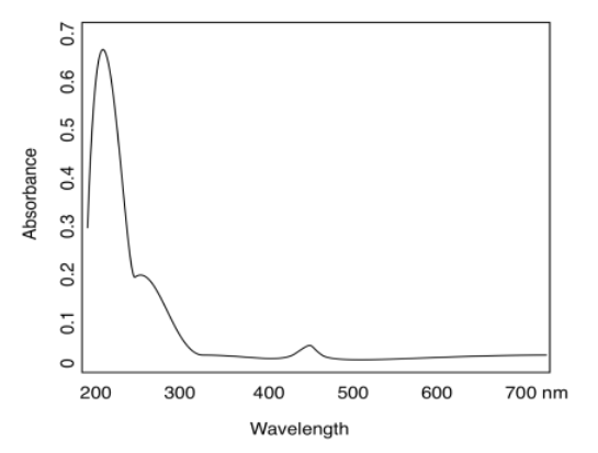
Ejercicio 2.3.3:

a) aproximadamente 250 nm b) aproximadamente 280 nm

Ejercicio 2.3.4:

b) amarillo

Ejercicio 2.3.5: