5.4: Ejemplos de líneas de transmisión

A modo de ejemplo, y también porque incluso tiene cierta importancia práctica, veamos un tipo de línea de transmisión. Se llama stripline y parece Figura\(\PageIndex{1}\). Consiste en un conductor plano, ubicado entre dos planos de tierra. Está soportado por un dieléctrico aislante con constante dieléctrica\(\varepsilon\). Esto es algo así como la situación que encontrarías en una placa de PC multinivel, donde quizás las líneas de bus estarían funcionando en una capa interna con planos de tierra por encima y por debajo de ellas.

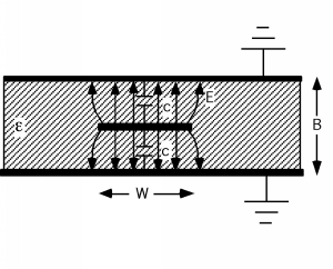Figura\(\PageIndex{1}\): Una línea de cinta

Entre el conductor central y el plano de tierra, habrá cierta capacitancia,\(C\). If we can assume that the electric field is more or less confined to the regions between the strip conductor and the ground plane (which occurs when the ratio of \(\frac{W}{B}\) is not too small), then for either capacitor (assuming unit length into the picture) we will get a value \[C = \frac{\varepsilon W}{\frac{B}{2}}\] since the value of a capacitor is just the dielectric constant times the area of the plates, divided by the spacing of the plates.

Looking quickly at Figure \(\PageIndex{1}\) you might think the two capacitors are in series, but you would be wrong! Note that each capacitor has one lead connected to the center conductor and the other lead connected to ground, and so the two capacitors are in fact in parallel, and hence their capacitances add. Thus, for the capacitance per unit length for this line, we can write: \[\mathbf{C} = \frac{4 \varepsilon W}{B}\]

It can be shown (although we won't do it here) that for any transmission line where the electric and magnetic fields are perpendicular to one another (called TEM or transverse electromagnetic) the speed of propagation of the wave down the line is just \[\begin{array}{l} v_{p} &= \dfrac{c}{\sqrt{\frac{\varepsilon}{\varepsilon_0}}} \\[4pt]   &= \dfrac{3 \times 10^{8} \ \frac{\mathrm{m}}{\mathrm{s}}}{\sqrt{\varepsilon_r}} \end{array}\]

where \(\varepsilon_{r}\) is called the relative dielectric constant for the material. Well, we also know that \[v_{p} = \frac{1}{\sqrt{\mathbf{LC}}}\]

From that, we can write \[\begin{array}{l} \mathbf{L} &= \dfrac{1}{v_{p}{ }^{2} \mathbf{C}} \\[4pt]   &= \dfrac{B}{v_{p}{ }^{2} 4 \varepsilon W} \end{array}\]

We can now insert this value for \(\mathbf{L}\) into the expression for \(Z_{0}\), the impedance of the line. \[\begin{array}{l} Z_{0} &= \sqrt{\dfrac{\mathbf{L}}{\mathbf{C}}} \\   &= \sqrt{\dfrac{\frac{B}{v_{p}{ }^{2} 4 \varepsilon W}}{\frac{4 \varepsilon W}{B}}} \\   &= \dfrac{B}{4 \varepsilon W v_{p}} \\   &= \dfrac{B}{4 \varepsilon W \frac{c}{\sqrt{\varepsilon_r}}} \end{array}\]

And so, we have derived an equation for the impedance \(Z_{0}\) of the line in terms of the dimensions \(W\) and \(B\), the dielectric constant of the insulating material, \(\varepsilon\), and \(c\), the speed of light. How good is this expression, and in particular how good is our assumption that the electric field is all confined to the region under the conductor? Not so great, actually. See Figure \(\PageIndex{2}\).

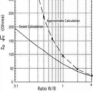
Figure \(\PageIndex{2}\): Exact and approximate \(Z_{0}\) for a stripline

Figure \(\PageIndex{2}\) shows the results from using Equation \(\PageIndex{6}\) and a more exact calculation, which takes into account the fringing fields. As you can see, we have to get the ratio \(\frac{W}{B}\) up to \(4\) or so before the two match. But at least we get the right behavior and we're not totally out of the ballpark.