6.5: Convolución Circular de Tiempo Continuo y el CTFS
- Page ID
- 86553
\( \newcommand{\vecs}[1]{\overset { \scriptstyle \rightharpoonup} {\mathbf{#1}} } \)
\( \newcommand{\vecd}[1]{\overset{-\!-\!\rightharpoonup}{\vphantom{a}\smash {#1}}} \)
\( \newcommand{\id}{\mathrm{id}}\) \( \newcommand{\Span}{\mathrm{span}}\)
( \newcommand{\kernel}{\mathrm{null}\,}\) \( \newcommand{\range}{\mathrm{range}\,}\)
\( \newcommand{\RealPart}{\mathrm{Re}}\) \( \newcommand{\ImaginaryPart}{\mathrm{Im}}\)
\( \newcommand{\Argument}{\mathrm{Arg}}\) \( \newcommand{\norm}[1]{\| #1 \|}\)
\( \newcommand{\inner}[2]{\langle #1, #2 \rangle}\)
\( \newcommand{\Span}{\mathrm{span}}\)
\( \newcommand{\id}{\mathrm{id}}\)
\( \newcommand{\Span}{\mathrm{span}}\)
\( \newcommand{\kernel}{\mathrm{null}\,}\)
\( \newcommand{\range}{\mathrm{range}\,}\)
\( \newcommand{\RealPart}{\mathrm{Re}}\)
\( \newcommand{\ImaginaryPart}{\mathrm{Im}}\)
\( \newcommand{\Argument}{\mathrm{Arg}}\)
\( \newcommand{\norm}[1]{\| #1 \|}\)
\( \newcommand{\inner}[2]{\langle #1, #2 \rangle}\)
\( \newcommand{\Span}{\mathrm{span}}\) \( \newcommand{\AA}{\unicode[.8,0]{x212B}}\)
\( \newcommand{\vectorA}[1]{\vec{#1}} % arrow\)
\( \newcommand{\vectorAt}[1]{\vec{\text{#1}}} % arrow\)
\( \newcommand{\vectorB}[1]{\overset { \scriptstyle \rightharpoonup} {\mathbf{#1}} } \)
\( \newcommand{\vectorC}[1]{\textbf{#1}} \)
\( \newcommand{\vectorD}[1]{\overrightarrow{#1}} \)
\( \newcommand{\vectorDt}[1]{\overrightarrow{\text{#1}}} \)
\( \newcommand{\vectE}[1]{\overset{-\!-\!\rightharpoonup}{\vphantom{a}\smash{\mathbf {#1}}}} \)
\( \newcommand{\vecs}[1]{\overset { \scriptstyle \rightharpoonup} {\mathbf{#1}} } \)
\( \newcommand{\vecd}[1]{\overset{-\!-\!\rightharpoonup}{\vphantom{a}\smash {#1}}} \)
\(\newcommand{\avec}{\mathbf a}\) \(\newcommand{\bvec}{\mathbf b}\) \(\newcommand{\cvec}{\mathbf c}\) \(\newcommand{\dvec}{\mathbf d}\) \(\newcommand{\dtil}{\widetilde{\mathbf d}}\) \(\newcommand{\evec}{\mathbf e}\) \(\newcommand{\fvec}{\mathbf f}\) \(\newcommand{\nvec}{\mathbf n}\) \(\newcommand{\pvec}{\mathbf p}\) \(\newcommand{\qvec}{\mathbf q}\) \(\newcommand{\svec}{\mathbf s}\) \(\newcommand{\tvec}{\mathbf t}\) \(\newcommand{\uvec}{\mathbf u}\) \(\newcommand{\vvec}{\mathbf v}\) \(\newcommand{\wvec}{\mathbf w}\) \(\newcommand{\xvec}{\mathbf x}\) \(\newcommand{\yvec}{\mathbf y}\) \(\newcommand{\zvec}{\mathbf z}\) \(\newcommand{\rvec}{\mathbf r}\) \(\newcommand{\mvec}{\mathbf m}\) \(\newcommand{\zerovec}{\mathbf 0}\) \(\newcommand{\onevec}{\mathbf 1}\) \(\newcommand{\real}{\mathbb R}\) \(\newcommand{\twovec}[2]{\left[\begin{array}{r}#1 \\ #2 \end{array}\right]}\) \(\newcommand{\ctwovec}[2]{\left[\begin{array}{c}#1 \\ #2 \end{array}\right]}\) \(\newcommand{\threevec}[3]{\left[\begin{array}{r}#1 \\ #2 \\ #3 \end{array}\right]}\) \(\newcommand{\cthreevec}[3]{\left[\begin{array}{c}#1 \\ #2 \\ #3 \end{array}\right]}\) \(\newcommand{\fourvec}[4]{\left[\begin{array}{r}#1 \\ #2 \\ #3 \\ #4 \end{array}\right]}\) \(\newcommand{\cfourvec}[4]{\left[\begin{array}{c}#1 \\ #2 \\ #3 \\ #4 \end{array}\right]}\) \(\newcommand{\fivevec}[5]{\left[\begin{array}{r}#1 \\ #2 \\ #3 \\ #4 \\ #5 \\ \end{array}\right]}\) \(\newcommand{\cfivevec}[5]{\left[\begin{array}{c}#1 \\ #2 \\ #3 \\ #4 \\ #5 \\ \end{array}\right]}\) \(\newcommand{\mattwo}[4]{\left[\begin{array}{rr}#1 \amp #2 \\ #3 \amp #4 \\ \end{array}\right]}\) \(\newcommand{\laspan}[1]{\text{Span}\{#1\}}\) \(\newcommand{\bcal}{\cal B}\) \(\newcommand{\ccal}{\cal C}\) \(\newcommand{\scal}{\cal S}\) \(\newcommand{\wcal}{\cal W}\) \(\newcommand{\ecal}{\cal E}\) \(\newcommand{\coords}[2]{\left\{#1\right\}_{#2}}\) \(\newcommand{\gray}[1]{\color{gray}{#1}}\) \(\newcommand{\lgray}[1]{\color{lightgray}{#1}}\) \(\newcommand{\rank}{\operatorname{rank}}\) \(\newcommand{\row}{\text{Row}}\) \(\newcommand{\col}{\text{Col}}\) \(\renewcommand{\row}{\text{Row}}\) \(\newcommand{\nul}{\text{Nul}}\) \(\newcommand{\var}{\text{Var}}\) \(\newcommand{\corr}{\text{corr}}\) \(\newcommand{\len}[1]{\left|#1\right|}\) \(\newcommand{\bbar}{\overline{\bvec}}\) \(\newcommand{\bhat}{\widehat{\bvec}}\) \(\newcommand{\bperp}{\bvec^\perp}\) \(\newcommand{\xhat}{\widehat{\xvec}}\) \(\newcommand{\vhat}{\widehat{\vvec}}\) \(\newcommand{\uhat}{\widehat{\uvec}}\) \(\newcommand{\what}{\widehat{\wvec}}\) \(\newcommand{\Sighat}{\widehat{\Sigma}}\) \(\newcommand{\lt}{<}\) \(\newcommand{\gt}{>}\) \(\newcommand{\amp}{&}\) \(\definecolor{fillinmathshade}{gray}{0.9}\)Introducción
Este módulo relaciona la convolución circular de señales periódicas en el dominio del tiempo con la multiplicación en el dominio de la frecuencia.
Convolución Circular de Señal
Dada una señal\(f(t)\) con coeficientes de Fourier\(c_n\) y una señal\(g(t)\) con coeficientes de Fourier\(d_n\), podemos definir una nueva señal,\(v(t)\), donde\(v(t)=f(t) \circledast g(t)\). Encontramos que la representación de la Serie de Fourier de\(v(t)\)\(a_n\),, es tal que\(a_n=c_nd_n\). \(f(t) \circledast g(t)\)es la convolución circular (Sección 7.5) de dos señales periódicas y es equivalente a la convolución en un intervalo, i.e\(f(t) \circledast g(t)=\int_{0}^{T} \int_{0}^{T} f(\tau) g(t-\tau) d \tau d t\).
Nota
La convolución circular en el dominio del tiempo es equivalente a la multiplicación de los coeficientes de Fourier.
Esto se demuestra de la siguiente manera
\ [\ begin {align}
a_ {n} &=\ frac {1} {T}\ int_ {0} ^ {T} v (t) e^ {-\ left (j\ omega_ {0} n t\ derecha)}\ mathrm {d} t\ nonumber\\
&=\ frac {1} {T^ {2}}\ int_ {0} ^ T}\ int_ {0} ^ {T} f (\ tau) g (t-\ tau)\ mathrm {d}\ tau e^ {-\ izquierda (\ omega j_ {0} n t\ derecha)}\ mathrm {d} t\ nonumber\\
&=\ frac {1} {T}\ int_ {0} ^ {T} f (\ tau)\ izquierda (\ frac {1} {T}\ int_ {0} ^ {T} g (t-\ tau) e^ {-\ izquierda (j\ omega_ {0} n t\ derecha)}\ mathrm {d} t\ derecha)\ mathrm {d}\ numbau\ er\\
&=\ forall\ nu,\ nu=t-\ ta u:\left (\ frac {1} {T}\ int_ {0} ^ {T} f (\ tau)\ izquierda (\ frac {1} {T}\ int_ {-\ tau} ^ {T-\ tau} g (\ nu) e^ {-\ izquierda (j\ omega_ {0} (\ nu=+\ tau)\ derecha)}\ mathrm {d}\ nu\ derecha)\ mathrm {d}\ tau\ derecha)\ nonumber\\
&=\ frac {1} {T} {T}\ int_ {0} ^ {T} f (\ tau)\ izquierda (\ frac {1} {T}\ int_ {-\ tau} ^ {T-\ tau} g (\ nu) e^ {-\ izquierda (j\ omega_ {0} n\ nu\ derecha)}\ mathrm {d}\ nu\ derecha) e^ {-\ izquierda (j\ omega_ {0} n\ tau\ derecha)}\ mathrm {d}\ tau\ nonumber\\
& amp; =\ frac {1} {T}\ int_ {0} ^ {T} f (\ tau) d_ {n} e^ {-\ izquierda (j\ omega_ {0} n\ tau\ derecha)}\ mathrm {d}\ tau\ nonumber\\
&=d_ {n}\ izquierda (\ frac {1} {T}\ int_ {0} ^ {T} f (\ tau) e^ {-\ izquierda (j\ omega_ {0} n\ tau\ derecha)}\ mathrm {d}\ tau\ derecha)\ nonumber\\
&=c_ {n} d_ {n}
\ end {align}\ nonumber\]
Ejercicio
Echa un vistazo a un pulso cuadrado con un periodo de\(T\).
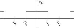
Para esta señal
\ [c_ {n} =\ izquierda\ {\ comenzar {matriz} {l}
\ frac {1} {T}\ texto {si} n=0\
\ frac {1} {2}\ frac {\ sin\ izquierda (\ frac {\ pi} {2} n\ derecha)} {\ frac {\ pi} {2} n}\ texto {de otro modo}
\ end {array}\ derecho. \ nonumber\]
Echa un vistazo a un tren de pulsos triangular con un periodo de\(T\).
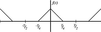
Esta señal se crea convolucionando circularmente el pulso cuadrado consigo mismo. Los coeficientes de Fourier para esta señal son\(a_{n}=c_{n}^{2}=\frac{1}{4} \frac{\sin ^{2}}{\left(\frac{\pi}{2} n\right)}\).
Ejercicio\(\PageIndex{1}\)
Encuentra los coeficientes de Fourier de la señal que se crea cuando se convoluciona el pulso cuadrado y el pulso triangular.
- Contestar
-
\ (a_ {n} =\ left\ {\ begin {array} {ll}
\ text {undefined} & n=0\\
\ frac {1} {8}\ frac {\ sin ^ {3}\ izquierda (\ frac {\ pi} {2} n\ derecha)} {\ izquierda (\ frac {\ pi} {2} n\ derecha) ^ {3}} &\ texto {de lo contrario}
\ end {array}\ right.\)
Conclusión
La convolución circular en el dominio del tiempo es equivalente a la multiplicación de los coeficientes de Fourier en el dominio de la frecuencia.