2.1: Vectores
- Page ID
- 113033

- Aprende a agregar y escalar vectores\(\mathbb{R}^n\text{,}\) tanto en álgebraica como geométricamente.
- Comprender las combinaciones lineales geométricamente.
- Imágenes: suma vectorial, resta vectorial, combinaciones lineales.
- Palabras de vocabulario: vector, combinación lineal.
Vectores en\(\mathbb{R}^n\)
Hemos estado dibujando puntos en\(\mathbb{R}^n\) como puntos en la línea, plano, espacio, etc. también podemos dibujarlos como flechas. Como tenemos en mente dos interpretaciones geométricas, ahora discutimos la relación entre los dos puntos de vista.
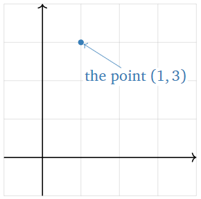
Nuevamente, un punto adentro\(\mathbb{R}^n\) se dibuja como un punto.
Figura\(\PageIndex{1}\)
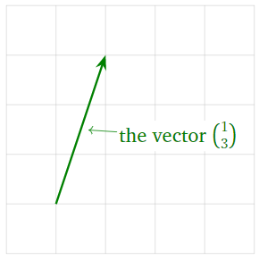
Un vector es un punto en\(\mathbb{R}^n\text{,}\) dibujado como una flecha.
Figura\(\PageIndex{2}\)
La diferencia es puramente psicológica: los puntos y los vectores son ambos solo listas de números.
When we think of a point in \(\mathbb{R}^n\) as a vector, we will usually write it vertically, like a matrix with one column:
\[v=\left(\begin{array}{c}1\\3\end{array}\right).\nonumber\]
We will also write \(0\) for the zero vector.
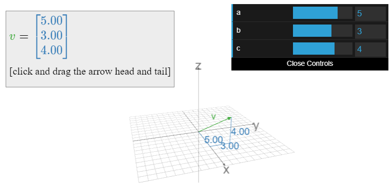
Why make the distinction between points and vectors? A vector need not start at the origin: it can be located anywhere! In other words, an arrow is determined by its length and its direction, not by its location. For instance, these arrows all represent the vector \(\color{green}{\left(\begin{array}{c}1\\2\end{array}\right)}\).
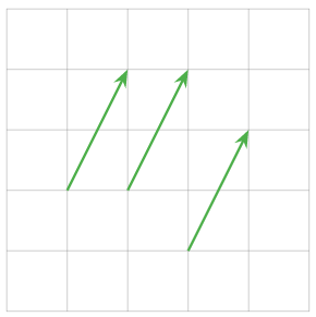
Figure \(\PageIndex{4}\)
Unless otherwise specified, we will assume that all vectors start at the origin.
Vectors makes sense in the real world: many physical quantities, such as velocity, are represented as vectors. But it makes more sense to think of the velocity of a car as being located at the car.
Some authors use boldface letters to represent vectors, as in “\(\mathbf v\)”, or use arrows, as in “\(\vec v\)”. As it is usually clear from context if a letter represents a vector, we do not decorate vectors in this way.
Another way to think about a vector is as a difference between two points, or the arrow from one point to another. For instance, \({1\choose 2}\) is the arrow from \((1,1)\) to \((2,3)\).
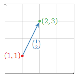
Figure \(\PageIndex{5}\)
Vector Algebra and Geometry
Here we learn how to add vectors together and how to multiply vectors by numbers, both algebraically and geometrically.
- We can add two vectors together:
\[\left(\begin{array}{c}a\\b\\c\end{array}\right) +\left(\begin{array}{c}x\\y\\z\end{array}\right)=\left(\begin{array}{c}a+x \\ b+y\\c+z\end{array}\right).\nonumber\] - We can multiply, or scale, a vector by a real number \(c\text{:}\)
\[\color{red}{c}\color{black}{\left(\begin{array}{c}x\\y\\z\end{array}\right)} =\left(\begin{array}{c}\color{red}{c}\color{black}{\:\cdot\: x} \\ \color{red}{c}\color{black}{\:\cdot\: y}\\ \color{red}{c}\color{black}{\:\cdot\: z}\end{array}\right).\nonumber\]
We call \(c\) a scalar to distinguish it from a vector. If \(v\) is a vector and \(c\) is a scalar, then \(cv\) is called a scalar multiple of \(v\).
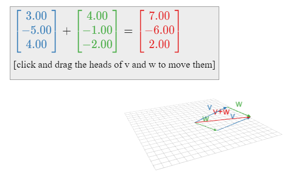
Addition and scalar multiplication work in the same way for vectors of length \(n\).
\[\left(\begin{array}{c}1\\2\\3\end{array}\right) +\left(\begin{array}{c}4\\5\\6\end{array}\right)=\left(\begin{array}{c}5\\7\\9\end{array}\right)\quad\text{and}\quad -2\left(\begin{array}{c}1\\2\\3\end{array}\right)=\left(\begin{array}{c}-2\\-4\\-6\end{array}\right).\nonumber\]
The Parallelogram Law for Vector Addition
Geometrically, the sum of two vectors \(v,w\) is obtained as follows: place the tail of \(w\) at the head of \(v\). Then \(v+w\) is the vector whose tail is the tail of \(v\) and whose head is the head of \(w\). Doing this both ways creates a parallelogram. For example,
\[\color{blue}{\left(\begin{array}{c}1\\3\end{array}\right)}\color{black}{+}\color{green}{\left(\begin{array}{c}4\\2\end{array}\right)}\color{black}{=\left(\begin{array}{c}5\\5\end{array}\right).}\nonumber\]
Why? The width of \(v+w\) is the sum of the widths, and likewise with the heights.
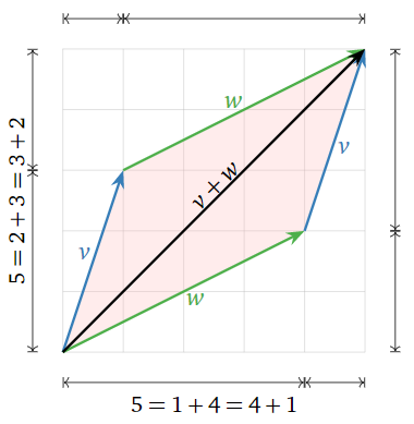
Figure \(\PageIndex{6}\)
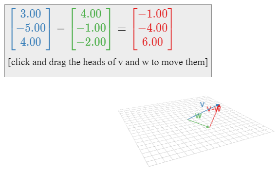
Vector Subtraction
Geometrically, the difference of two vectors \(v,w\) is obtained as follows: place the tail of \(v\) and \(w\) at the same point. Then \(v-w\) is the vector from the head of \(w\) to the head of \(v\). For example,
\[\color{blue}{\left(\begin{array}{c}1\\4\end{array}\right)}\color{black}{-}\color{green}{\left(\begin{array}{c}4\\2\end{array}\right)}\color{black}{=\left(\begin{array}{c}-3\\2\end{array}\right).}\nonumber\]
Why? If you add \(v-w\) to \(w\text{,}\) you get \(v\).
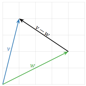
Figure \(\PageIndex{8}\)
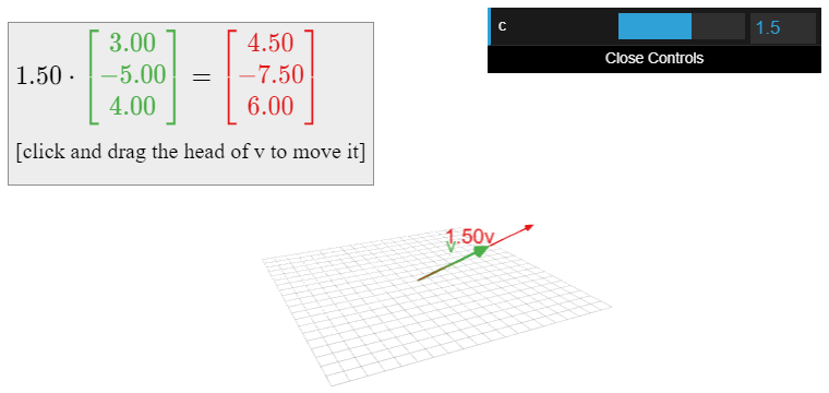
Scalar Multiplication
A scalar multiple of a vector \(v\) has the same (or opposite) direction, but a different length. For instance, \(2v\) is the vector in the direction of \(v\) but twice as long, and \(-\frac 12v\) is the vector in the opposite direction of \(v\text{,}\) but half as long. Note that the set of all scalar multiples of a (nonzero) vector \(v\) is a line.
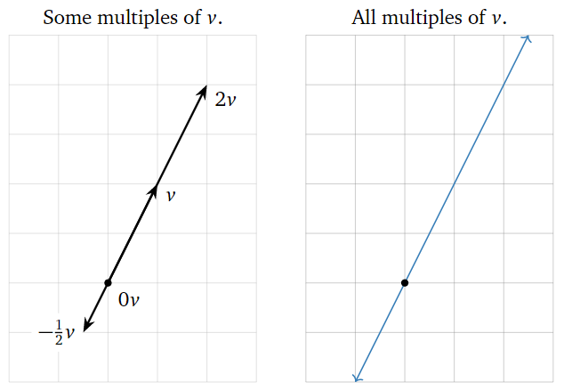
Figure \(\PageIndex{10}\)
Combinaciones Lineales
Podemos agregar y escalar vectores en la misma ecuación.
\(c_1,c_2,\ldots,c_k\)Dejen ser escalares, y dejar que\(v_1,v_2,\ldots,v_k\) sean vectores adentro\(\mathbb{R}^n\). El vector en\(\mathbb{R}^n\)
\[ c_1v_1 + c_2v_2 + \cdots + c_kv_k \nonumber \]
se llama una combinación lineal de los vectores\(v_1,v_2,\ldots,v_k\text{,}\) con pesos o coeficientes\(c_1,c_2,\ldots,c_k\).
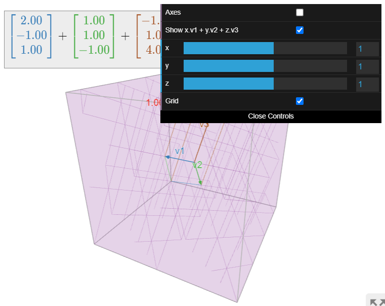
Geométricamente, se obtiene una combinación lineal estirando/encogiendo los vectores\(v_1,v_2,\ldots,v_k\) según los coeficientes, luego sumarlos usando la ley del paralelogramo.
Dejar\(v_1 = {1\choose 2}\) y\(v_2 = {1\choose 0}\). Aquí hay algunas combinaciones lineales de\(v_1\) y\(v_2\text{,}\) dibujadas como puntos.
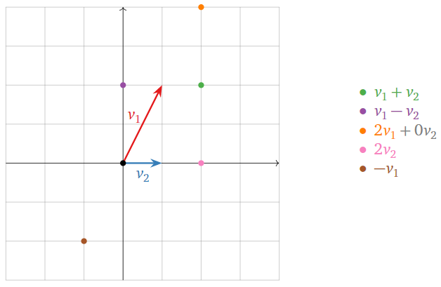
Figura\(\PageIndex{12}\)
Las ubicaciones de estos puntos se encuentran utilizando la ley de paralelogramo para la adición de vectores. Cualquier vector en el plano es una combinación lineal de\(v_1\) y\(v_2\text{,}\) con coeficientes adecuados.
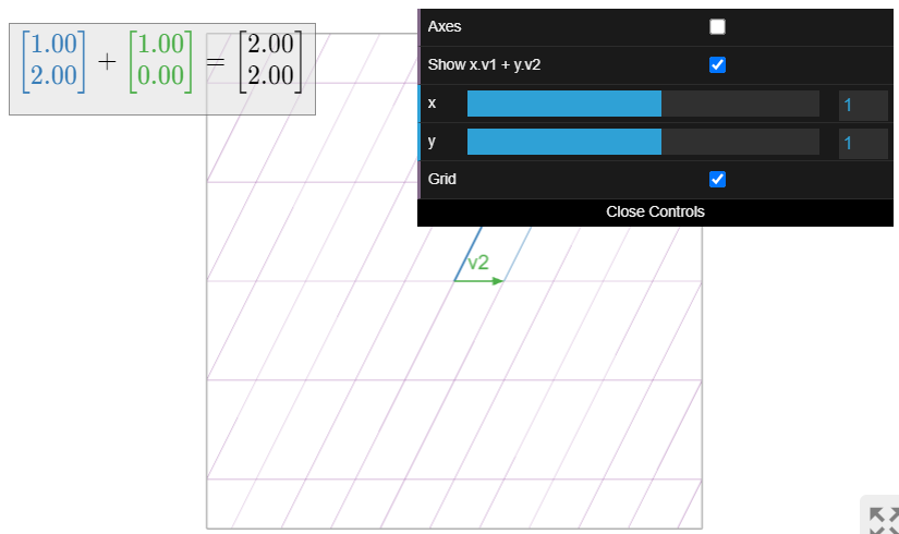
Figura\(\PageIndex{13}\): Combinaciones lineales de dos vectores en\(\mathbb{R}^2\text{:}\) movimiento los deslizadores para cambiar los coeficientes de\(v_1\) y\(v_2\). Tenga en cuenta que cualquier vector en el plano se puede obtener como una combinación lineal de\(v_1,v_2\) con coeficientes adecuados.
A linear combination of a single vector \(v = {1\choose 2}\) is just a scalar multiple of \(v\). So some examples include
\[v=\left(\begin{array}{c}1\\2\end{array}\right),\quad \frac{3}{2}v=\left(\begin{array}{c}3/2\\3\end{array}\right),\quad -\frac{1}{2}v=\left(\begin{array}{c}-1/2\\-1\end{array}\right),\quad\cdots\nonumber\]
The set of all linear combinations is the line through \(v\). (Unless \(v=0\text{,}\) in which case any scalar multiple of \(v\) is again \(0\).)
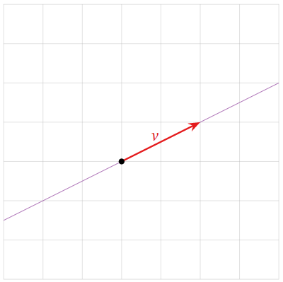
Figure \(\PageIndex{15}\)
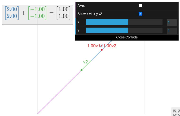
The set of all linear combinations of the vectors
\[v_{1}=\left(\begin{array}{c}2\\2\end{array}\right)\quad\text{and}\quad v_{2}=\left(\begin{array}{c}-1\\-1\end{array}\right)\nonumber\]
is the line containing both vectors.
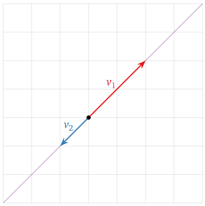
Figure \(\PageIndex{16}\)
The difference between this and Example \(\PageIndex{6}\) is that both vectors lie on the same line. Hence any scalar multiples of \(v_1,v_2\) lie on that line, as does their sum.