
6.2: Complementos ortogonales
- Page ID
- 113101

\( \newcommand{\vecs}[1]{\overset { \scriptstyle \rightharpoonup} {\mathbf{#1}} } \)
\( \newcommand{\vecd}[1]{\overset{-\!-\!\rightharpoonup}{\vphantom{a}\smash {#1}}} \)
\( \newcommand{\dsum}{\displaystyle\sum\limits} \)
\( \newcommand{\dint}{\displaystyle\int\limits} \)
\( \newcommand{\dlim}{\displaystyle\lim\limits} \)
\( \newcommand{\id}{\mathrm{id}}\) \( \newcommand{\Span}{\mathrm{span}}\)
( \newcommand{\kernel}{\mathrm{null}\,}\) \( \newcommand{\range}{\mathrm{range}\,}\)
\( \newcommand{\RealPart}{\mathrm{Re}}\) \( \newcommand{\ImaginaryPart}{\mathrm{Im}}\)
\( \newcommand{\Argument}{\mathrm{Arg}}\) \( \newcommand{\norm}[1]{\| #1 \|}\)
\( \newcommand{\inner}[2]{\langle #1, #2 \rangle}\)
\( \newcommand{\Span}{\mathrm{span}}\)
\( \newcommand{\id}{\mathrm{id}}\)
\( \newcommand{\Span}{\mathrm{span}}\)
\( \newcommand{\kernel}{\mathrm{null}\,}\)
\( \newcommand{\range}{\mathrm{range}\,}\)
\( \newcommand{\RealPart}{\mathrm{Re}}\)
\( \newcommand{\ImaginaryPart}{\mathrm{Im}}\)
\( \newcommand{\Argument}{\mathrm{Arg}}\)
\( \newcommand{\norm}[1]{\| #1 \|}\)
\( \newcommand{\inner}[2]{\langle #1, #2 \rangle}\)
\( \newcommand{\Span}{\mathrm{span}}\) \( \newcommand{\AA}{\unicode[.8,0]{x212B}}\)
\( \newcommand{\vectorA}[1]{\vec{#1}} % arrow\)
\( \newcommand{\vectorAt}[1]{\vec{\text{#1}}} % arrow\)
\( \newcommand{\vectorB}[1]{\overset { \scriptstyle \rightharpoonup} {\mathbf{#1}} } \)
\( \newcommand{\vectorC}[1]{\textbf{#1}} \)
\( \newcommand{\vectorD}[1]{\overrightarrow{#1}} \)
\( \newcommand{\vectorDt}[1]{\overrightarrow{\text{#1}}} \)
\( \newcommand{\vectE}[1]{\overset{-\!-\!\rightharpoonup}{\vphantom{a}\smash{\mathbf {#1}}}} \)
\( \newcommand{\vecs}[1]{\overset { \scriptstyle \rightharpoonup} {\mathbf{#1}} } \)
\(\newcommand{\longvect}{\overrightarrow}\)
\( \newcommand{\vecd}[1]{\overset{-\!-\!\rightharpoonup}{\vphantom{a}\smash {#1}}} \)
\(\newcommand{\avec}{\mathbf a}\) \(\newcommand{\bvec}{\mathbf b}\) \(\newcommand{\cvec}{\mathbf c}\) \(\newcommand{\dvec}{\mathbf d}\) \(\newcommand{\dtil}{\widetilde{\mathbf d}}\) \(\newcommand{\evec}{\mathbf e}\) \(\newcommand{\fvec}{\mathbf f}\) \(\newcommand{\nvec}{\mathbf n}\) \(\newcommand{\pvec}{\mathbf p}\) \(\newcommand{\qvec}{\mathbf q}\) \(\newcommand{\svec}{\mathbf s}\) \(\newcommand{\tvec}{\mathbf t}\) \(\newcommand{\uvec}{\mathbf u}\) \(\newcommand{\vvec}{\mathbf v}\) \(\newcommand{\wvec}{\mathbf w}\) \(\newcommand{\xvec}{\mathbf x}\) \(\newcommand{\yvec}{\mathbf y}\) \(\newcommand{\zvec}{\mathbf z}\) \(\newcommand{\rvec}{\mathbf r}\) \(\newcommand{\mvec}{\mathbf m}\) \(\newcommand{\zerovec}{\mathbf 0}\) \(\newcommand{\onevec}{\mathbf 1}\) \(\newcommand{\real}{\mathbb R}\) \(\newcommand{\twovec}[2]{\left[\begin{array}{r}#1 \\ #2 \end{array}\right]}\) \(\newcommand{\ctwovec}[2]{\left[\begin{array}{c}#1 \\ #2 \end{array}\right]}\) \(\newcommand{\threevec}[3]{\left[\begin{array}{r}#1 \\ #2 \\ #3 \end{array}\right]}\) \(\newcommand{\cthreevec}[3]{\left[\begin{array}{c}#1 \\ #2 \\ #3 \end{array}\right]}\) \(\newcommand{\fourvec}[4]{\left[\begin{array}{r}#1 \\ #2 \\ #3 \\ #4 \end{array}\right]}\) \(\newcommand{\cfourvec}[4]{\left[\begin{array}{c}#1 \\ #2 \\ #3 \\ #4 \end{array}\right]}\) \(\newcommand{\fivevec}[5]{\left[\begin{array}{r}#1 \\ #2 \\ #3 \\ #4 \\ #5 \\ \end{array}\right]}\) \(\newcommand{\cfivevec}[5]{\left[\begin{array}{c}#1 \\ #2 \\ #3 \\ #4 \\ #5 \\ \end{array}\right]}\) \(\newcommand{\mattwo}[4]{\left[\begin{array}{rr}#1 \amp #2 \\ #3 \amp #4 \\ \end{array}\right]}\) \(\newcommand{\laspan}[1]{\text{Span}\{#1\}}\) \(\newcommand{\bcal}{\cal B}\) \(\newcommand{\ccal}{\cal C}\) \(\newcommand{\scal}{\cal S}\) \(\newcommand{\wcal}{\cal W}\) \(\newcommand{\ecal}{\cal E}\) \(\newcommand{\coords}[2]{\left\{#1\right\}_{#2}}\) \(\newcommand{\gray}[1]{\color{gray}{#1}}\) \(\newcommand{\lgray}[1]{\color{lightgray}{#1}}\) \(\newcommand{\rank}{\operatorname{rank}}\) \(\newcommand{\row}{\text{Row}}\) \(\newcommand{\col}{\text{Col}}\) \(\renewcommand{\row}{\text{Row}}\) \(\newcommand{\nul}{\text{Nul}}\) \(\newcommand{\var}{\text{Var}}\) \(\newcommand{\corr}{\text{corr}}\) \(\newcommand{\len}[1]{\left|#1\right|}\) \(\newcommand{\bbar}{\overline{\bvec}}\) \(\newcommand{\bhat}{\widehat{\bvec}}\) \(\newcommand{\bperp}{\bvec^\perp}\) \(\newcommand{\xhat}{\widehat{\xvec}}\) \(\newcommand{\vhat}{\widehat{\vvec}}\) \(\newcommand{\uhat}{\widehat{\uvec}}\) \(\newcommand{\what}{\widehat{\wvec}}\) \(\newcommand{\Sighat}{\widehat{\Sigma}}\) \(\newcommand{\lt}{<}\) \(\newcommand{\gt}{>}\) \(\newcommand{\amp}{&}\) \(\definecolor{fillinmathshade}{gray}{0.9}\)- Comprender las propiedades básicas de los complementos ortogonales.
- Aprender a calcular el complemento ortogonal de un subespacio.
- Recetas: atajos para computar los complementos ortogonales de los subespacios comunes.
- Imagen: complementos ortogonales en\(\mathbb{R}^2 \) y\(\mathbb{R}^3 \).
- Teorema: rango de fila es igual al rango de columna.
- Palabras de vocabulario: complemento ortogonal, espacio de filas.
Será importante calcular el conjunto de todos los vectores que son ortogonales a un conjunto dado de vectores. Resulta que un vector es ortogonal a un conjunto de vectores si y sólo si es ortogonal al lapso de esos vectores, que es un subespacio, por lo que nos limitamos al caso de los subespacios.
Definición del Complemento Ortogonal
Tomar el complemento ortogonal es una operación que se realiza en subespacios.
Que\(W\) sea un subespacio de\(\mathbb{R}^n \). Su complemento ortogonal es el subespacio
\[ W^\perp = \bigl\{ \text{$v$ in $\mathbb{R}^n $}\mid v\cdot w=0 \text{ for all $w$ in $W$} \bigr\}. \nonumber \]
El símbolo a veces\(W^\perp\) se lee “\(W\)perp”.
Este es el conjunto de todos los vectores\(v\) en\(\mathbb{R}^n \) que son ortogonales a todos los vectores en\(W\). Mostraremos a continuación 15 que efectivamente\(W^\perp\) es un subespacio.
Ahora tenemos dos piezas de notación de aspecto similar:
\[ \begin{split} A^{\color{Red}T} \amp\text{ is the transpose of a matrix $A$}. \\ W^{\color{Red}\perp} \amp\text{ is the orthogonal complement of a subspace $W$}. \end{split} \nonumber \]
Trate de no confundir a los dos.
Imágenes de complementos ortogonales
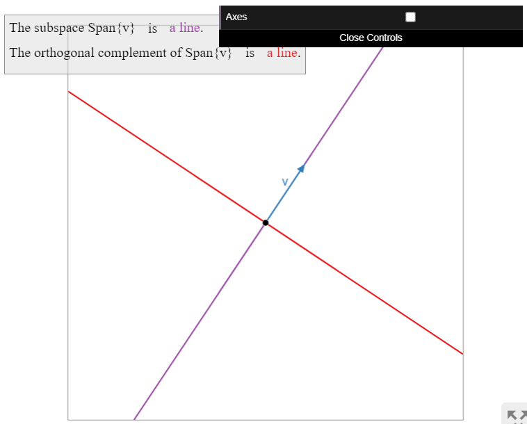
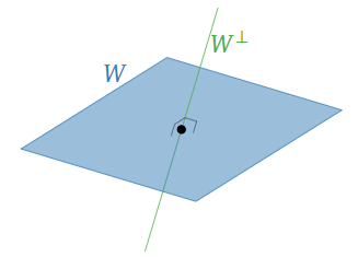
El complemento ortogonal de una línea\(\color{blue}W\) a través del origen en\(\mathbb{R}^2 \) es la línea perpendicular\(\color{Green}W^\perp\).
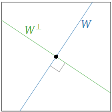
Figura\(\PageIndex{1}\)
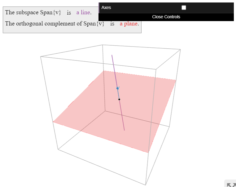
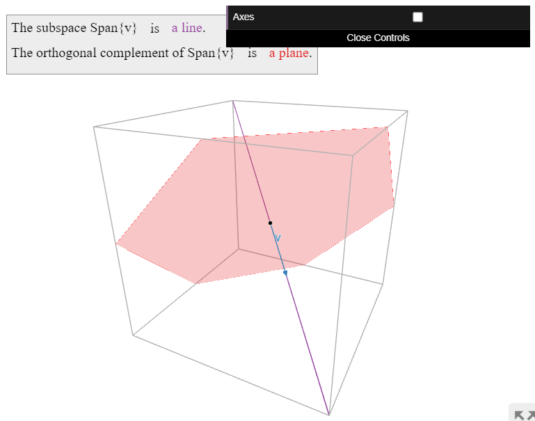
The orthogonal complement of a line \(\color{blue}W\) in \(\mathbb{R}^3 \) is the perpendicular plane \(\color{Green}W^\perp\).
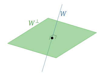
Figure \(\PageIndex{3}\)
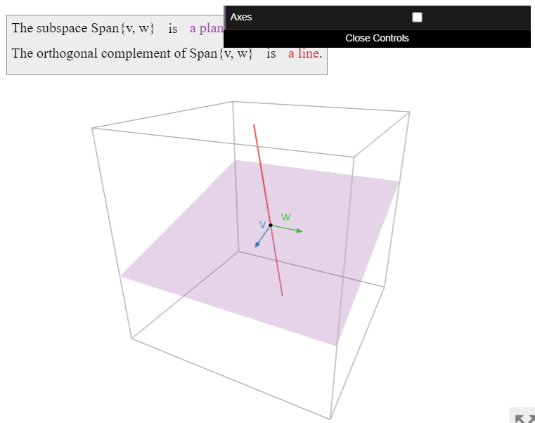
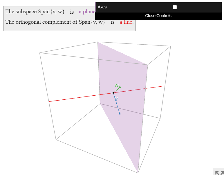
El complemento ortogonal de un plano\(\color{blue}W\) en\(\mathbb{R}^3 \) es la línea perpendicular\(\color{Green}W^\perp\).
Figura\(\PageIndex{5}\)
We see in the above pictures that \((W^\perp)^\perp = W\).
The orthogonal complement of \(\mathbb{R}^n \) is \(\{0\}\text{,}\) since the zero vector is the only vector that is orthogonal to all of the vectors in \(\mathbb{R}^n \).
For the same reason, we have \(\{0\}^\perp = \mathbb{R}^n \).
Computing Orthogonal Complements
Since any subspace is a span, the following proposition gives a recipe for computing the orthogonal complement of any subspace. However, below we will give several shortcuts for computing the orthogonal complements of other common kinds of subspaces–in particular, null spaces. To compute the orthogonal complement of a general subspace, usually it is best to rewrite the subspace as the column space or null space of a matrix, as in Note 2.6.3 in Section 2.6.
Let \(A\) be a matrix and let \(W=\text{Col}(A)\). Then
\[ W^\perp = \text{Nul}(A^T). \nonumber \]
- Proof
-
To justify the first equality, we need to show that a vector \(x\) is perpendicular to the all of the vectors in \(W\) if and only if it is perpendicular only to \(v_1,v_2,\ldots,v_m\). Since the \(v_i\) are contained in \(W\text{,}\) we really only have to show that if \(x\cdot v_1 = x\cdot v_2 = \cdots = x\cdot v_m = 0\text{,}\) then \(x\) is perpendicular to every vector \(v\) in \(W\). Indeed, any vector in \(W\) has the form \(v = c_1v_1 + c_2v_2 + \cdots + c_mv_m\) for suitable scalars \(c_1,c_2,\ldots,c_m\text{,}\) so
\[ \begin{split} x\cdot v \amp= x\cdot(c_1v_1 + c_2v_2 + \cdots + c_mv_m) \\ \amp= c_1(x\cdot v_1) + c_2(x\cdot v_2) + \cdots + c_m(x\cdot v_m) \\ \amp= c_1(0) + c_2(0) + \cdots + c_m(0) = 0. \end{split} \nonumber \]
Therefore, \(x\) is in \(W^\perp.\)
To prove the second equality, we let
\[ A = \left(\begin{array}{c}—v_1^T— \\ —v_2^T— \\ \vdots \\ —v_m^T—\end{array}\right). \nonumber \]
By the row-column rule for matrix multiplication Definition 2.3.3 in Section 2.3, for any vector \(x\) in \(\mathbb{R}^n \) we have
\[ Ax = \left(\begin{array}{c}v_1^Tx \\ v_2^Tx\\ \vdots\\ v_m^Tx\end{array}\right) = \left(\begin{array}{c}v_1\cdot x\\ v_2\cdot x\\ \vdots \\ v_m\cdot x\end{array}\right). \nonumber \]
Therefore, \(x\) is in \(\text{Nul}(A)\) if and only if \(x\) is perpendicular to each vector \(v_1,v_2,\ldots,v_m\).
Since column spaces are the same as spans, we can rephrase the proposition as follows. Let \(v_1,v_2,\ldots,v_m\) be vectors in \(\mathbb{R}^n \text{,}\) and let \(W = \text{Span}\{v_1,v_2,\ldots,v_m\}\). Then
\[ W^\perp = \bigl\{\text{all vectors orthogonal to each $v_1,v_2,\ldots,v_m$}\bigr\} = \text{Nul}\left(\begin{array}{c}—v_1^T— \\ —v_2^T— \\ \vdots \\ —v_m^T—\end{array}\right). \nonumber \]
Again, it is important to be able to go easily back and forth between spans and column spaces. If you are handed a span, you can apply the proposition once you have rewritten your span as a column space.
By the proposition, computing the orthogonal complement of a span means solving a system of linear equations. For example, if
\[ v_1 = \left(\begin{array}{c}1\\7\\2\end{array}\right) \qquad v_2 = \left(\begin{array}{c}-2\\3\\1\end{array}\right) \nonumber \]
then \(\text{Span}\{v_1,v_2\}^\perp\) is the solution set of the homogeneous linear system associated to the matrix
\[ \left(\begin{array}{c}—v_1^T— \\ —v_2^T—\end{array}\right) = \left(\begin{array}{ccc}1&7&2\\-2&3&1\end{array}\right). \nonumber \]
This is the solution set of the system of equations
\[\left\{\begin{array}{rrrrrrr}x_1 &+& 7x_2 &+& 2x_3 &=& 0\\ -2x_1 &+& 3x_2 &+& x_3 &=&0.\end{array}\right.\nonumber\]
Compute \(W^\perp\text{,}\) where
\[ W = \text{Span}\left\{\left(\begin{array}{c}1\\7\\2\end{array}\right),\;\left(\begin{array}{c}-2\\3\\1\end{array}\right)\right\}. \nonumber \]
Solution
According to Proposition \(\PageIndex{1}\), we need to compute the null space of the matrix
\[ \left(\begin{array}{ccc}1&7&2\\-2&3&1\end{array}\right) \;\xrightarrow{\text{RREF}}\; \left(\begin{array}{ccc}1&0&-1/17 \\ 0&1&5/17\end{array}\right). \nonumber \]
The free variable is \(x_3\text{,}\) so the parametric form of the solution set is \(x_1=x_3/17,\,x_2=-5x_3/17\text{,}\) and the parametric vector form is
\[ \left(\begin{array}{c}x_1\\x_2\\x_3\end{array}\right) = x_3\left(\begin{array}{c}1/17 \\ -5/17\\1\end{array}\right). \nonumber \]
Scaling by a factor of \(17\text{,}\) we see that
\[ W^\perp = \text{Span}\left\{\left(\begin{array}{c}1\\-5\\17\end{array}\right)\right\}. \nonumber \]
We can check our work:
\[ \left(\begin{array}{c}1\\7\\2\end{array}\right)\cdot\left(\begin{array}{c}1\\-5\\17\end{array}\right) = 0 \qquad \left(\begin{array}{c}-2\\3\\1\end{array}\right)\cdot\left(\begin{array}{c}1\\-5\\17\end{array}\right) = 0. \nonumber \]
Find all vectors orthogonal to \(v = \left(\begin{array}{c}1\\1\\-1\end{array}\right).\)
Solution
According to Proposition \(\PageIndex{1}\), we need to compute the null space of the matrix
\[ A = \left(\begin{array}{c}—v—\end{array}\right) = \left(\begin{array}{ccc}1&1&-1\end{array}\right). \nonumber \]
This matrix is in reduced-row echelon form. The parametric form for the solution set is \(x_1 = -x_2 + x_3\text{,}\) so the parametric vector form of the general solution is
\[ x = \left(\begin{array}{c}x_1\\x_2\\x_3\end{array}\right) = x_2\left(\begin{array}{c}-1\\1\\0\end{array}\right) + x_3\left(\begin{array}{c}1\\0\\1\end{array}\right). \nonumber \]
Therefore, the answer is the plane
\[ \text{Span}\left\{\left(\begin{array}{c}-1\\1\\0\end{array}\right),\;\left(\begin{array}{c}1\\0\\1\end{array}\right)\right\}. \nonumber \]
Compute
\[ \text{Span}\left\{\left(\begin{array}{c}1\\1\\-1\end{array}\right),\;\left(\begin{array}{c}1\\1\\1\end{array}\right)\right\}^\perp. \nonumber \]
Solution
According to Proposition \(\PageIndex{1}\), we need to compute the null space of the matrix
\[ A = \left(\begin{array}{ccc}1&1&-1\\1&1&1\end{array}\right)\;\xrightarrow{\text{RREF}}\;\left(\begin{array}{ccc}1&1&0\\0&0&1\end{array}\right). \nonumber \]
The parametric vector form of the solution is
\[ \left(\begin{array}{c}x_1\\x_2\\x_3\end{array}\right) = x_2\left(\begin{array}{c}-1\\1\\0\end{array}\right). \nonumber \]
Therefore, the answer is the line
\[ \text{Span}\left\{\left(\begin{array}{c}-1\\1\\0\end{array}\right)\right\}. \nonumber \]
In order to find shortcuts for computing orthogonal complements, we need the following basic facts. Looking back the the above examples, all of these facts should be believable.
Let \(W\) be a subspace of \(\mathbb{R}^n \). Then:
- \(W^\perp\) is also a subspace of \(\mathbb{R}^n .\)
- \((W^\perp)^\perp = W.\)
- \(\dim(W) + \dim(W^\perp) = n.\)
- Proof
-
For the first assertion, we verify the three defining properties of subspaces, Definition 2.6.2 in Section 2.6.
- The zero vector is in \(W^\perp\) because the zero vector is orthogonal to every vector in \(\mathbb{R}^n \).
- Let \(u,v\) be in \(W^\perp\text{,}\) so \(u\cdot x = 0\) and \(v\cdot x = 0\) for every vector \(x\) in \(W\). We must verify that \((u+v)\cdot x = 0\) for every \(x\) in \(W\). Indeed, we have \[ (u+v)\cdot x = u\cdot x + v\cdot x = 0 + 0 = 0. \nonumber \]
- Let \(u\) be in \(W^\perp\text{,}\) so \(u\cdot x = 0\) for every \(x\) in \(W\text{,}\) and let \(c\) be a scalar. We must verify that \((cu)\cdot x = 0\) for every \(x\) in \(W\). Indeed, we have \[ (cu)\cdot x = c(u\cdot x) = c0 = 0. \nonumber \]
Next we prove the third assertion. Let \(v_1,v_2,\ldots,v_m\) be a basis for \(W\text{,}\) so \(m = \dim(W)\text{,}\) and let \(v_{m+1},v_{m+2},\ldots,v_k\) be a basis for \(W^\perp\text{,}\) so \(k-m = \dim(W^\perp)\). We need to show \(k=n\). First we claim that \(\{v_1,v_2,\ldots,v_m,v_{m+1},v_{m+2},\ldots,v_k\}\) is linearly independent. Suppose that \(c_1v_1 + c_2v_2 + \cdots + c_kv_k = 0\). Let \(w = c_1v_1 + c_2v_2 + \cdots + c_mv_m\) and \(w' = c_{m+1}v_{m+1} + c_{m+2}v_{m+2} + \cdots + c_kv_k\text{,}\) so \(w\) is in \(W\text{,}\) \(w'\) is in \(W'\text{,}\) and \(w + w' = 0\). Then \(w = -w'\) is in both \(W\) and \(W^\perp\text{,}\) which implies \(w\) is perpendicular to itself. In particular, \(w\cdot w = 0\text{,}\) so \(w = 0\text{,}\) and hence \(w' = 0\). Therefore, all coefficients \(c_i\) are equal to zero, because \(\{v_1,v_2,\ldots,v_m\}\) and \(\{v_{m+1},v_{m+2},\ldots,v_k\}\) are linearly independent.
It follows from the previous paragraph that \(k \leq n\). Suppose that \(k \lt n\). Then the matrix
\[ A = \left(\begin{array}{c}—v_1^T— \\ —v_2^T— \\ \vdots \\ —v_k^T—\end{array}\right) \nonumber \]
has more columns than rows (it is “wide”), so its null space is nonzero by Note 3.2.1 in Section 3.2. Let \(x\) be a nonzero vector in \(\text{Nul}(A)\). Then
\[ 0 = Ax = \left(\begin{array}{c}v_1^Tx \\ v_2^Tx \\ \vdots \\ v_k^Tx\end{array}\right) = \left(\begin{array}{c}v_1\cdot x\\ v_2\cdot x\\ \vdots \\ v_k\cdot x\end{array}\right) \nonumber \]
by the row-column rule for matrix multiplication Definition 2.3.3 in Section 2.3. Since \(v_1\cdot x = v_2\cdot x = \cdots = v_m\cdot x = 0\text{,}\) it follows from Proposition \(\PageIndex{1}\) that \(x\) is in \(W^\perp\text{,}\) and similarly, \(x\) is in \((W^\perp)^\perp\). As above, this implies \(x\) is orthogonal to itself, which contradicts our assumption that \(x\) is nonzero. Therefore, \(k = n\text{,}\) as desired.
Finally, we prove the second assertion. Clearly \(W\) is contained in \((W^\perp)^\perp\text{:}\) this says that everything in \(W\) is perpendicular to the set of all vectors perpendicular to everything in \(W\). Let \(m=\dim(W).\) By 3, we have \(\dim(W^\perp) = n-m\text{,}\) so \(\dim((W^\perp)^\perp) = n - (n-m) = m\). The only \(m\)-dimensional subspace of \((W^\perp)^\perp\) is all of \((W^\perp)^\perp\text{,}\) so \((W^\perp)^\perp = W.\)
See subsection Pictures of orthogonal complements, for pictures of the second property. As for the third: for example, if \(W\) is a (\(2\)-dimensional) plane in \(\mathbb{R}^4\text{,}\) then \(W^\perp\) is another (\(2\)-dimensional) plane. Explicitly, we have
\[\begin{aligned}\text{Span}\{e_1,e_2\}^{\perp}&=\left\{\left(\begin{array}{c}x\\y\\z\\w\end{array}\right)\text{ in }\mathbb{R}\left| \left(\begin{array}{c}x\\y\\z\\w\end{array}\right)\cdot\left(\begin{array}{c}1\\0\\0\\0\end{array}\right)=0\text{ and }\left(\begin{array}{c}x\\y\\z\\w\end{array}\right)\left(\begin{array}{c}0\\1\\0\\0\end{array}\right)=0\right.\right\} \\ &=\left\{\left(\begin{array}{c}0\\0\\z\\w\end{array}\right)\text{ in }\mathbb{R}^4\right\}=\text{Span}\{e_3,e_4\}:\end{aligned}\]
the orthogonal complement of the \(xy\)-plane is the \(zw\)-plane.
The row space of a matrix \(A\) is the span of the rows of \(A\text{,}\) and is denoted \(\text{Row}(A)\).
If \(A\) is an \(m\times n\) matrix, then the rows of \(A\) are vectors with \(n\) entries, so \(\text{Row}(A)\) is a subspace of \(\mathbb{R}^n \). Equivalently, since the rows of \(A\) are the columns of \(A^T\text{,}\) the row space of \(A\) is the column space of \(A^T\text{:}\)
\[ \text{Row}(A) = \text{Col}(A^T). \nonumber \]
We showed in the above Proposition \(\PageIndex{3}\) that if \(A\) has rows \(v_1^T,v_2^T,\ldots,v_m^T\text{,}\) then
\[ \text{Row}(A)^\perp = \text{Span}\{v_1,v_2,\ldots,v_m\}^\perp = \text{Nul}(A). \nonumber \]
Taking orthogonal complements of both sides and using the second fact \(\PageIndex{1}\) gives
\[ \text{Row}(A) = \text{Nul}(A)^\perp. \nonumber \]
Replacing \(A\) by \(A^T\) and remembering that \(\text{Row}(A)=\text{Col}(A^T)\) gives
\[ \text{Col}(A)^\perp = \text{Nul}(A^T) \quad\text{and}\quad \text{Col}(A) = \text{Nul}(A^T)^\perp. \nonumber \]
To summarize:
For any vectors \(v_1,v_2,\ldots,v_m\text{,}\) we have
\[ \text{Span}\{v_1,v_2,\ldots,v_m\}^\perp = \text{Nul}\left(\begin{array}{c}—v_1^T— \\ —v_2^T— \\ \vdots \\ —v_m^T—\end{array}\right) . \nonumber \]
For any matrix \(A\text{,}\) we have
\[ \begin{aligned} \text{Row}(A)^\perp &= \text{Nul}(A) & \text{Nul}(A)^\perp &= \text{Row}(A) \\ \text{Col}(A)^\perp &= \text{Nul}(A^T)\quad & \text{Nul}(A^T)^\perp &= \text{Col}(A). \end{aligned} \nonumber \]
As mentioned in the beginning of this subsection, in order to compute the orthogonal complement of a general subspace, usually it is best to rewrite the subspace as the column space or null space of a matrix.
Compute the orthogonal complement of the subspace
\[ W = \bigl\{(x,y,z) \text{ in } \mathbb{R}^3 \mid 3x + 2y = z\bigr\}. \nonumber \]
Solution
Rewriting, we see that \(W\) is the solution set of the system of equations \(3x + 2y - z = 0\text{,}\) i.e., the null space of the matrix \(A = \left(\begin{array}{ccc}3&2&-1\end{array}\right).\) Therefore,
\[ W^\perp = \text{Row}(A) = \text{Span}\left\{\left(\begin{array}{c}3\\2\\-1\end{array}\right)\right\}. \nonumber \]
No row reduction was needed!
Find the orthogonal complement of the \(5\)-eigenspace of the matrix
\[A=\left(\begin{array}{ccc}2&4&-1\\3&2&0\\-2&4&3\end{array}\right).\nonumber\]
Solution
The \(5\)-eigenspace is
\[ W = \text{Nul}(A - 5I_3) = \text{Nul}\left(\begin{array}{ccc}-3&4&-1\\3&-3&0\\-2&4&-2\end{array}\right), \nonumber \]
so
\[ W^\perp = \text{Row}\left(\begin{array}{ccc}-3&4&-1\\3&-3&0\\-2&4&-2\end{array}\right) = \text{Span}\left\{\left(\begin{array}{c}-3\\4\\-1\end{array}\right),\;\left(\begin{array}{c}3\\-3\\0\end{array}\right),\;\left(\begin{array}{c}-2\\4\\-2\end{array}\right)\right\}. \nonumber \]
These vectors are necessarily linearly dependent (why)?
Row rank and Column Rank
Suppose that \(A\) is an \(m \times n\) matrix. Let us refer to the dimensions of \(\text{Col}(A)\) and \(\text{Row}(A)\) as the row rank and the column rank of \(A\) (note that the column rank of \(A\) is the same as the rank of \(A\)). The next theorem says that the row and column ranks are the same. This is surprising for a couple of reasons. First, \(\text{Row}(A)\) lies in \(\mathbb{R}^n \) and \(\text{Col}(A)\) lies in \(\mathbb{R}^m \). Also, the theorem implies that \(A\) and \(A^T\) have the same number of pivots, even though the reduced row echelon forms of \(A\) and \(A^T\) have nothing to do with each other otherwise.
Let \(A\) be a matrix. Then the row rank of \(A\) is equal to the column rank of \(A\).
- Proof
-
By Theorem 2.9.1 in Section 2.9, we have
\[ \dim\text{Col}(A) + \dim\text{Nul}(A) = n. \nonumber \]
On the other hand the third fact \(\PageIndex{1}\) says that
\[ \dim\text{Nul}(A)^\perp + \dim\text{Nul}(A) = n, \nonumber \]
which implies \(\dim\text{Col}(A) = \dim\text{Nul}(A)^\perp\). Since \(\text{Nul}(A)^\perp = \text{Row}(A),\) we have
\[ \dim\text{Col}(A) = \dim\text{Row}(A)\text{,} \nonumber \]
as desired.
In particular, by Corollary 2.7.1 in Section 2.7 both the row rank and the column rank are equal to the number of pivots of \(A\).