
6.3: Proyección ortogonal
- Page ID
- 113092

- Comprender la descomposición ortogonal de un vector con respecto a un subespacio.
- Comprender la relación entre la descomposición ortogonal y la proyección ortogonal.
- Comprender la relación entre la descomposición ortogonal y el vector más cercano en/distancia a un subespacio.
- Aprender las propiedades básicas de las proyecciones ortogonales como transformaciones lineales y como transformaciones matriciales.
- Recetas: proyección ortogonal sobre una línea, descomposición ortogonal mediante la resolución de un sistema de ecuaciones, proyección ortogonal a través de un producto matricial complicado.
- Imágenes: descomposición ortogonal, proyección ortogonal.
- Palabras de vocabulario: descomposición ortogonal, proyección ortogonal.
Dejar\(W\) ser un subespacio de\(\mathbb{R}^n \) y dejar\(x\) ser un vector en\(\mathbb{R}^n \). En esta sección, aprenderemos a calcular el vector más cercano\(x_W\) a\(x\) in\(W\). El vector\(x_W\) se llama la proyección ortogonal de\(x\) sobre\(W\). Esto es exactamente lo que vamos a utilizar para resolver casi ecuaciones matriciales, como se discute en la introducción al Capítulo 6.
Descomposición ortogonal
Comenzamos fijando alguna notación.
Dejar\(W\) ser un subespacio de\(\mathbb{R}^n \) y dejar\(x\) ser un vector en\(\mathbb{R}^n \). Denotamos el vector más cercano a\(x\) on\(W\) by\(x_W\).
Decir que\(x_W\) es el vector más cercano a\(x\) on\(W\) significa que la diferencia\(x-x_W\) es ortogonal a los vectores en\(W\text{:}\)
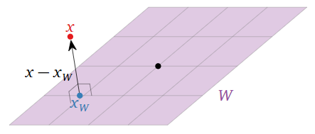
Figura\(\PageIndex{1}\)
En otras palabras, si\(x_{W^\perp} = x - x_W\text{,}\) entonces tenemos\(x = x_W + x_{W^\perp}\text{,}\) dónde\(x_W\) está adentro\(W\) y\(x_{W^\perp}\) está adentro\(W^\perp\). El primer orden del día es demostrar que el vector más cercano siempre existe.
Dejar\(W\) ser un subespacio de\(\mathbb{R}^n \) y dejar\(x\) ser un vector en\(\mathbb{R}^n \). Entonces podemos escribir de\(x\) manera única como
\[ x = x_W + x_{W^\perp} \nonumber \]
donde\(x_W\) es el vector más cercano a\(x\) on\(W\) y\(x_{W^\perp}\) está adentro\(W^\perp\).
- Prueba
-
Que\(m = \dim(W)\text{,}\) así\(n-m = \dim(W^\perp)\) por Hecho 6.2.1 en la Sección 6.2. Seamos\(v_1,v_2,\ldots,v_m\) una base para\(W\) y dejemos\(v_{m+1},v_{m+2},\ldots,v_n\) ser una base para\(W^\perp\). Mostramos en la prueba de este Hecho 6.2.1 en la Sección 6.2 que\(\{v_1,v_2,\ldots,v_m,v_{m+1},v_{m+2},\ldots,v_n\}\) es linealmente independiente, por lo que forma una base para\(\mathbb{R}^n \). Por lo tanto, podemos escribir
\[ x = (c_1v_1 + \cdots + c_mv_m) + (c_{m+1}v_{m+1} + \cdots + c_nv_n) = x_W + x_{W^\perp}, \nonumber \]
dónde\(x_W = c_1v_1 + \cdots + c_mv_m\) y\(x_{W^\perp} = c_{m+1}v_{m+1} + \cdots + c_nv_n\). Dado que\(x_{W^\perp}\) es ortogonal\(W\text{,}\) al vector\(x_W\) es el vector más cercano a\(x\) on\(W\text{,}\) por lo que esto demuestra que existe tal descomposición.
En cuanto a la singularidad, supongamos que
\[ x = x_W + x_{W^\perp} = y_W + y_{W^\perp} \nonumber \]
para\(x_W,y_W\) dentro\(W\) y\(x_{W^\perp},y_{W^\perp}\) en\(W^\perp\). Reorganizar da
\[ x_W - y_W = y_{W^\perp} - x_{W^\perp}. \nonumber \]
Dado que\(W\) y\(W^\perp\) son subespacios, el lado izquierdo de la ecuación está adentro\(W\) y el lado derecho está adentro\(W^\perp\). Por lo tanto,\(x_W-y_W\) está en\(W\) y en\(W^\perp\text{,}\) lo que es ortogonal a sí mismo, lo que implica\(x_W-y_W=0\). De ahí\(x_W = y_W\) y\(x_{W^\perp} = y_{W^\perp}\text{,}\) que demuestra singularidad.
Dejar\(W\) ser un subespacio de\(\mathbb{R}^n \) y dejar\(x\) ser un vector en\(\mathbb{R}^n \). La expresión
\[ x = x_W + x_{W^\perp} \nonumber \]
for\(x_W\) in\(W\) y\(x_{W^\perp}\) in\(W^\perp\text{,}\) se llama la descomposición ortogonal de\(x\) con respecto a\(W\text{,}\) y el vector más cercano\(x_W\) es la proyección ortogonal de\(x\) sobre\(W\).
Dado que\(x_W\) es el vector más cercano\(W\) a\(x\text{,}\) la distancia desde\(x\) el subespacio\(W\) es la longitud del vector desde\(x_W\) hasta\(x\text{,}\) es decir, la longitud de\(x_{W^\perp}\). Para reafirmar:
Dejar\(W\) ser un subespacio de\(\mathbb{R}^n \) y dejar\(x\) ser un vector en\(\mathbb{R}^n \).
- La proyección ortogonal\(x_W\) es el vector más cercano a\(x\) in\(W\).
- La distancia de\(x\) a\(W\) es\(\|x_{W^\perp}\|\).
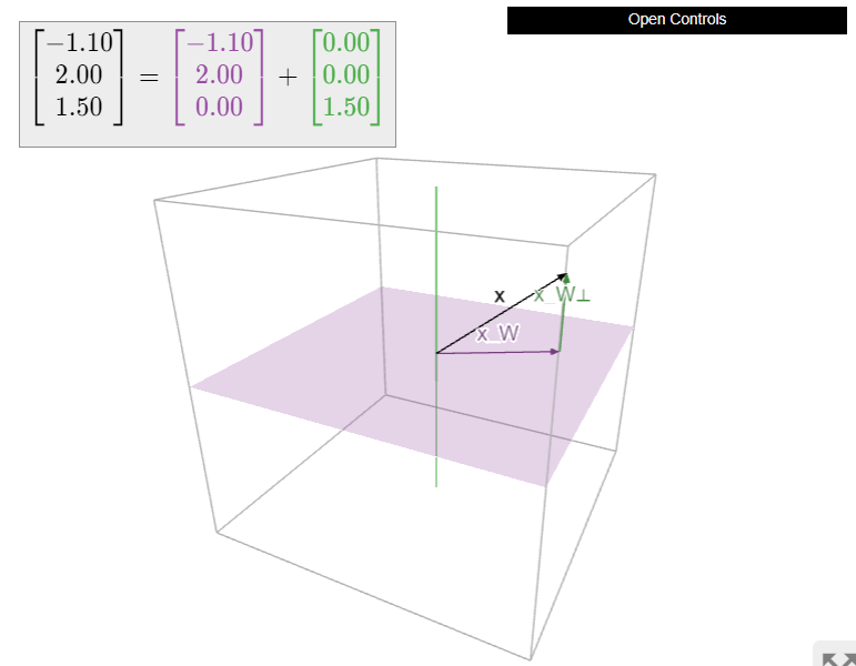
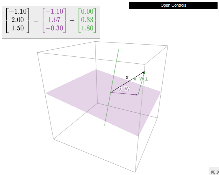
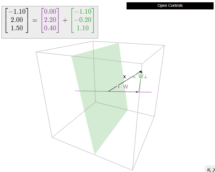
Dejar\(W\) ser el\(xy\) -plano en\(\mathbb{R}^3 \text{,}\) así\(W^\perp\) es el\(z\) eje -. Es fácil calcular la descomposición ortogonal de un vector con respecto a esto\(W\text{:}\)
\[\begin{aligned}x&=\left(\begin{array}{c}1\\2\\3\end{array}\right)\implies x_W=\left(\begin{array}{c}1\\2\\0\end{array}\right)\:\:x_{W^{\perp}}=\left(\begin{array}{c}0\\0\\3\end{array}\right) \\ x&=\left(\begin{array}{c}a\\b\\c\end{array}\right)\implies x_W=\left(\begin{array}{c}a\\b\\0\end{array}\right)\:\:x_{W^{\perp}}=\left(\begin{array}{c}0\\0\\c\end{array}\right).\end{aligned}\]
Vemos que la descomposición ortogonal en este caso expresa un vector en términos de un componente “horizontal” (en el\(xy\) plano) y un componente “vertical” (en el\(z\) eje).
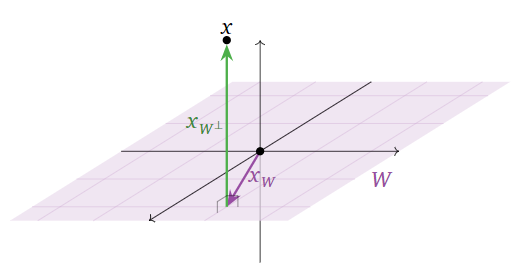
Figura\(\PageIndex{2}\)
Si\(x\) está en un subespacio\(W\text{,}\) entonces el vector más cercano a\(x\) in\(W\) es en sí mismo, así\(x = x_W\) y\(x_{W^\perp} = 0\). Por el contrario, si\(x = x_W\) entonces\(x\) está contenido en\(W\) porque\(x_W\) está contenido en\(W\).
Si\(W\) es un subespacio y\(x\) está en\(W^\perp\text{,}\) entonces la descomposición ortogonal de\(x\) es\(x = 0 + x\text{,}\) donde\(0\) está adentro\(W\) y\(x\) está adentro\(W^\perp\). De ello se deduce que\(x_W = 0\). Por el contrario, si\(x_W = 0\) entonces la descomposición ortogonal de\(x\) es\(x = x_W + x_{W^\perp} = 0 + x_{W^\perp}\text{,}\) así\(x = x_{W^\perp}\) está en\(W^\perp\).
Now we turn to the problem of computing \(x_W\) and \(x_{W^\perp}\). Of course, since \(x_{W^\perp} = x - x_W\text{,}\) really all we need is to compute \(x_W\). The following theorem gives a method for computing the orthogonal projection onto a column space. To compute the orthogonal projection onto a general subspace, usually it is best to rewrite the subspace as the column space of a matrix, as in Note 2.6.3 in Section 2.6.
Let \(A\) be an \(m \times n\) matrix, let \(W = \text{Col}(A)\text{,}\) and let \(x\) be a vector in \(\mathbb{R}^m \). Then the matrix equation
\[ A^TAc=A^Tx \nonumber \]
in the unknown vector \(c\) is consistent, and \(x_W\) is equal to \(Ac\) for any solution \(c\).
- Proof
-
Let \(x = x_W + x_{W^\perp}\) be the orthogonal decomposition with respect to \(W\). By definition \(x_W\) lies in \(W=\text{Col}(A)\) and so there is a vector \(c\) in \(\mathbb{R}^n \) with \(Ac = x_W\). Choose any such vector \(c\). We know that \(x-x_W=x-Ac\) lies in \(W^\perp\text{,}\) which is equal to \(\text{Nul}(A^T)\) by Recipe: Shortcuts for Computing Orthogonal Complements in Section 6.2. We thus have
\[ 0=A^T(x-Ac) = A^Tx-A^TAc \nonumber \]
and so
\[ A^TAc = A^Tx. \nonumber \]
This exactly means that \(A^TAc = A^Tx\) is consistent. If \(c\) is any solution to \(A^TAc=A^Tx\) then by reversing the above logic, we conclude that \(x_W = Ac\).
Let \(L = \text{Span}\{u\}\) be a line in \(\mathbb{R}^n \) and let \(x\) be a vector in \(\mathbb{R}^n \). By Theorem \(\PageIndex{2}\), to find \(x_L\) we must solve the matrix equation \(u^Tuc = u^Tx\text{,}\) where we regard \(u\) as an \(n\times 1\) matrix (the column space of this matrix is exactly \(L\text{!}\)). But \(u^Tu = u\cdot u\) and \(u^Tx = u\cdot x\text{,}\) so \(c = (u\cdot x)/(u\cdot u)\) is a solution of \(u^Tuc = u^Tx\text{,}\) and hence \(x_L = uc = (u\cdot x)/(u\cdot u)\,u.\)
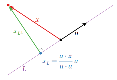
Figure \(\PageIndex{7}\)
To reiterate:
If \(L = \text{Span}\{u\}\) is a line, then
\[ x_L = \frac{u\cdot x}{u\cdot u}\,u \quad\text{and}\quad x_{L^\perp} = x - x_L \nonumber \]
for any vector \(x\).
In the special case where we are projecting a vector \(x\) in \(\mathbb{R}^n \) onto a line \(L = \text{Span}\{u\}\text{,}\) our formula for the projection can be derived very directly and simply. The vector \(x_L\) is a multiple of \(u\text{,}\) say \(x_L=cu\). This multiple is chosen so that \(x-x_L=x-cu\) is perpendicular to \(u\text{,}\) as in the following picture.
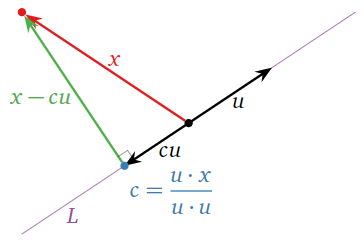
Figure \(\PageIndex{8}\)
In other words,
\[ (x-cu) \cdot u = 0. \nonumber \]
Using the distributive property for the dot product and isolating the variable \(c\) gives us that
\[ c = \frac{u\cdot x}{u\cdot u} \nonumber \]
and so
\[ x_L = cu = \frac{u\cdot x}{u\cdot u}\,u. \nonumber \]
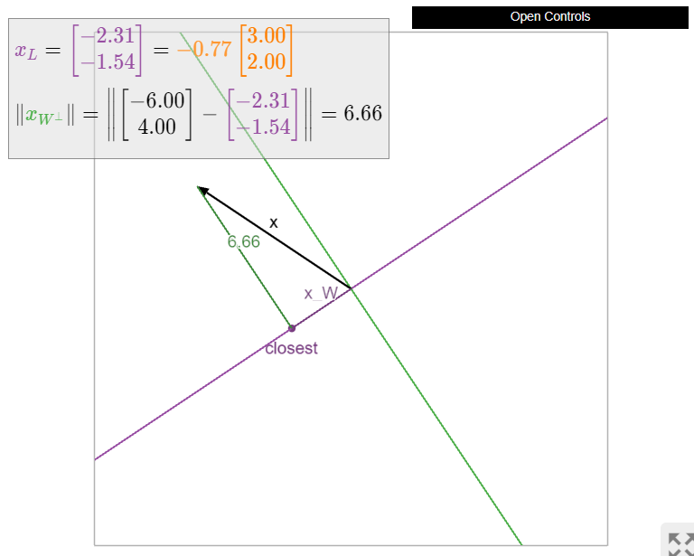
Compute the orthogonal projection of \(x = {-6\choose 4}\) onto the line \(L\) spanned by \(u = {3\choose 2}\text{,}\) and find the distance from \(x\) to \(L\).
Solution
First we find
\[ x_L = \frac{x\cdot u}{u\cdot u}\,u = \frac{-18+8}{9+4}\left(\begin{array}{c}3\\2\end{array}\right) = -\frac{10}{13}\left(\begin{array}{c}3\\2\end{array}\right) \qquad x_{L^\perp} = x - x_L = \frac 1{13}\left(\begin{array}{c}-48\\72\end{array}\right). \nonumber \]
The distance from \(x\) to \(L\) is
\[ \|x_{L^\perp}\| = \frac 1{13}\sqrt{48^2 + 72^2} \approx 6.656. \nonumber \]
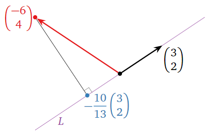
Figure \(\PageIndex{9}\)
Let
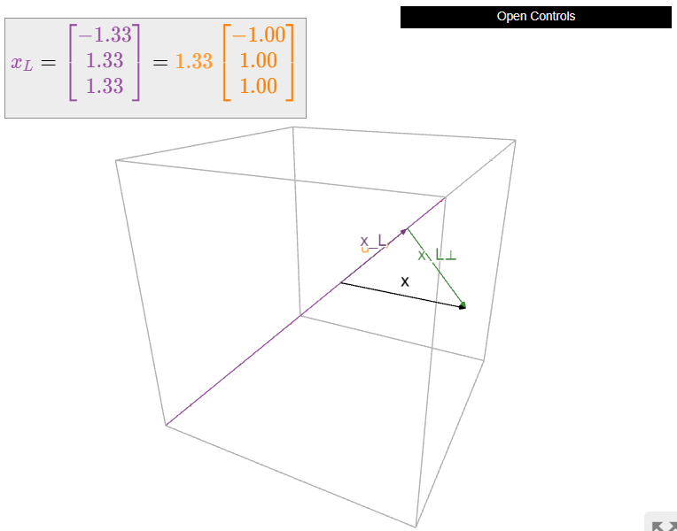
\[ x = \left(\begin{array}{c}-2\\3\\-1\end{array}\right) \qquad u = \left(\begin{array}{c}-1\\1\\1\end{array}\right), \nonumber \]
and let \(L\) be the line spanned by \(u\). Compute \(x_L\) and \(x_L^\perp\).
Solution
\[ x_L = \frac{x\cdot u}{u\cdot u}\,u = \frac{2+3-1}{1+1+1}\left(\begin{array}{c}-1\\1\\1\end{array}\right) = \frac{4}{3}\left(\begin{array}{c}-1\\1\\1\end{array}\right) \qquad x_{L^\perp} = x - x_L = \frac 13\left(\begin{array}{c}-2\\5\\-7\end{array}\right). \nonumber \]
When \(A\) is a matrix with more than one column, computing the orthogonal projection of \(x\) onto \(W = \text{Col}(A)\) means solving the matrix equation \(A^TAc = A^Tx\). In other words, we can compute the closest vector by solving a system of linear equations. To be explicit, we state Theorem \(\PageIndex{2}\) as a recipe:
Let \(W\) be a subspace of \(\mathbb{R}^m \). Here is a method to compute the orthogonal decomposition of a vector \(x\) with respect to \(W\text{:}\)
- Rewrite \(W\) as the column space of a matrix \(A\). In other words, find a a spanning set for \(W\text{,}\) and let \(A\) be the matrix with those columns.
- Compute the matrix \(A^TA\) and the vector \(A^Tx\).
- Form the augmented matrix for the matrix equation \(A^TAc = A^Tx\) in the unknown vector \(c\text{,}\) and row reduce.
- This equation is always consistent; choose one solution \(c\). Then \[ x_W = Ac \qquad x_{W^\perp} = x - x_W. \nonumber \]
Use Theorem \(\PageIndex{2}\) to compute the orthogonal decomposition of a vector with respect to the \(xy\)-plane in \(\mathbb{R}^3 \).
Solution
A basis for the \(xy\)-plane is given by the two standard coordinate vectors
\[ e_1 = \left(\begin{array}{c}1\\0\\0\end{array}\right) \qquad e_2 =\left(\begin{array}{c}0\\1\\0\end{array}\right). \nonumber \]
Let \(A\) be the matrix with columns \(e_1,e_2\text{:}\)
\[ A = \left(\begin{array}{cc}1&0\\0&1\\0&0\end{array}\right). \nonumber \]
Then
\[ A^TA = \left(\begin{array}{cc}1&0\\0&1\end{array}\right) = I_2 \qquad A^T\left(\begin{array}{c}x_1\\x_2\\x_3\end{array}\right) = \left(\begin{array}{ccc}1&0&0\\0&1&0\end{array}\right)\left(\begin{array}{c}x_1\\x_2\\x_3\end{array}\right) = \left(\begin{array}{c}x_1\\x_2\end{array}\right). \nonumber \]
It follows that the unique solution \(c\) of \(A^TAc = I_2c = A^Tx\) is given by the first two coordinates of \(x\text{,}\) so
\[ x_W = A\left(\begin{array}{c}x_1\\x_2\end{array}\right) = \left(\begin{array}{cc}1&0\\0&1\\0&0\end{array}\right)\left(\begin{array}{c}x_1\\x_2\end{array}\right) = \left(\begin{array}{c}x_1\\x_2\\0\end{array}\right) \qquad x_{W^\perp} = x - x_W = \left(\begin{array}{c}0\\0\\x_3\end{array}\right). \nonumber \]
We have recovered this Example \(\PageIndex{1}\).
Let
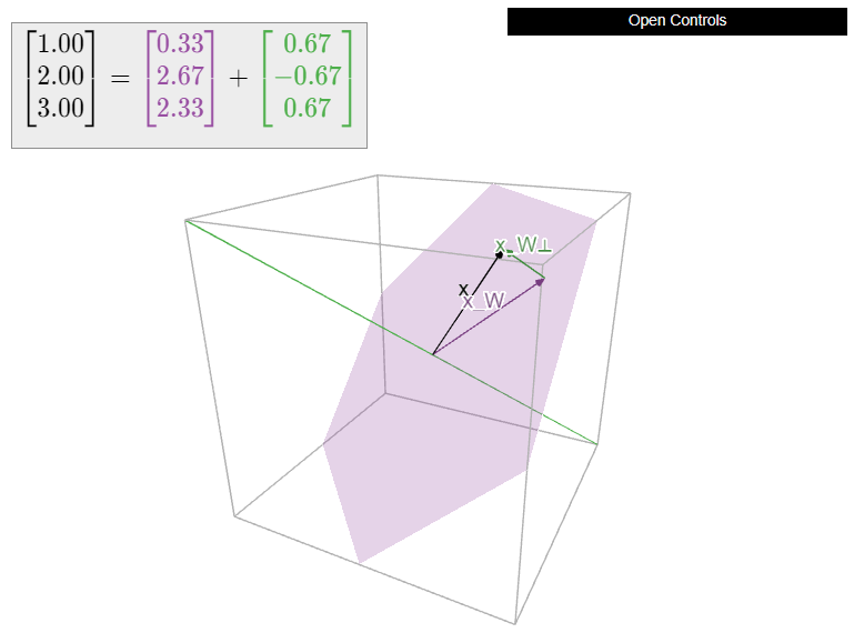
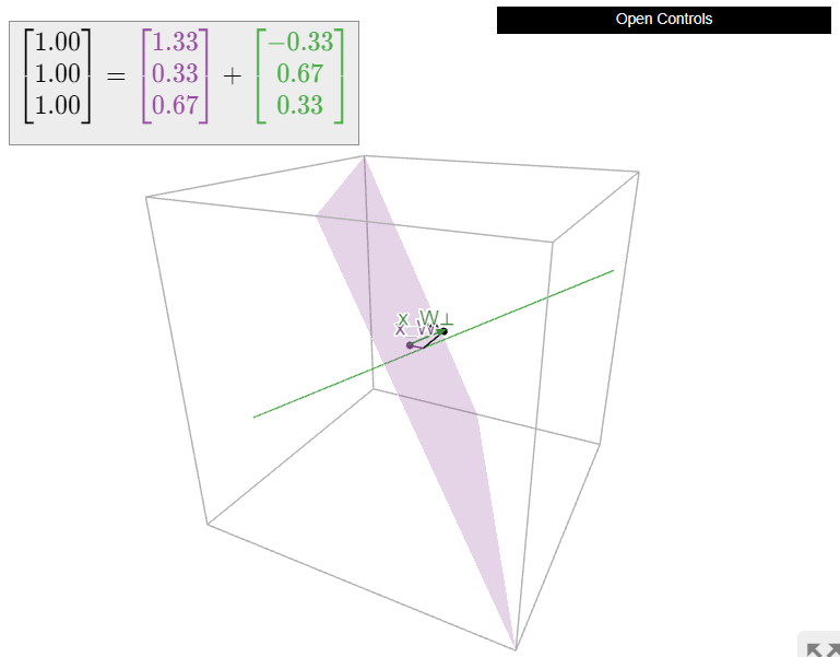
\[ W = \text{Span}\left\{\left(\begin{array}{c}1\\0\\-1\end{array}\right),\;\left(\begin{array}{c}1\\1\\0\end{array}\right)\right\} \qquad x = \left(\begin{array}{c}1\\2\\3\end{array}\right). \nonumber \]
Compute \(x_W\) and the distance from \(x\) to \(W\).
Solution
We have to solve the matrix equation \(A^TAc = A^Tx\text{,}\) where
\[ A = \left(\begin{array}{cc}1&1\\0&1\\-1&0\end{array}\right). \nonumber \]
We have
\[ A^TA = \left(\begin{array}{cc}2&1\\1&2\end{array}\right) \qquad A^Tx = \left(\begin{array}{c}-2\\3\end{array}\right). \nonumber \]
We form an augmented matrix and row reduce:
\[ \left(\begin{array}{cc|c}2&1&-2\\1&2&3\end{array}\right)\xrightarrow{\text{RREF}}\left(\begin{array}{cc|c} 1&0&-7/3 \\ 0&1&8/3\end{array}\right) \implies c = \frac 13\left(\begin{array}{c}-7\\8\end{array}\right). \nonumber \]
It follows that
\[ x_W = Ac = \frac 13\left(\begin{array}{c}1\\8\\7\end{array}\right) \qquad x_{W^\perp} = x - x_W = \frac 13\left(\begin{array}{c}2\\-2\\2\end{array}\right). \nonumber \]
The distance from \(x\) to \(W\) is
\[ \|x_{W^\perp}\| = \frac 1{3}\sqrt{4+4+4} \approx 1.155. \nonumber \]
Let
\[ W = \left\{\left(\begin{array}{c}x_1\\x_2\\x_3\end{array}\right)\bigm|x_1 - 2x_2 = x_3\right\} \quad\text{and}\quad x = \left(\begin{array}{c}1\\1\\1\end{array}\right). \nonumber \]
Compute \(x_W\).
Solution
Method 1: First we need to find a spanning set for \(W\). We notice that \(W\) is the solution set of the homogeneous equation \(x_1 - 2x_2 - x_3 = 0\text{,}\) so \(W = \text{Nul}\left(\begin{array}{ccc}1&-2&-1\end{array}\right)\). We know how to compute a basis for a null space: we row reduce and find the parametric vector form. The matrix \(\left(\begin{array}{ccc}1&-2&-1\end{array}\right)\) is already in reduced row echelon form. The parametric form is \(x_1 = 2x_2 + x_3\text{,}\) so the parametric vector form is
\[ \left(\begin{array}{c}x_1\\x_2\\x_3\end{array}\right) = x_2\left(\begin{array}{c}2\\1\\0\end{array}\right) + x_3\left(\begin{array}{c}1\\0\\1\end{array}\right), \nonumber \]
and hence a basis for \(V\) is given by
\[ \left\{\left(\begin{array}{c}2\\1\\0\end{array}\right),\;\left(\begin{array}{c}1\\0\\1\end{array}\right)\right\}. \nonumber \]
We let \(A\) be the matrix whose columns are our basis vectors:
\[ A = \left(\begin{array}{cc}2&1\\1&0\\0&1\end{array}\right). \nonumber \]
Hence \(\text{Col}(A) = \text{Nul}\left(\begin{array}{ccc}1&-2&-1\end{array}\right) = W\).
Now we can continue with step 1 of the recipe. We compute
\[ A^TA = \left(\begin{array}{cc}5&2\\2&2\end{array}\right) \qquad A^Tx = \left(\begin{array}{c}3\\2\end{array}\right). \nonumber \]
We write the linear system \(A^TAc = A^Tx\) as an augmented matrix and row reduce:
\[ \left(\begin{array}{cc|c}5&2&3\\2&2&2\end{array}\right)\xrightarrow{\text{RREF}}\left(\begin{array}{cc|c}1&0&1/3 \\ 0&1&2/3\end{array}\right). \nonumber \]
Hence we can take \(c = {1/3\choose 2/3}\text{,}\) so
\[ x_W = Ac =\left(\begin{array}{cc}2&1\\1&0\\0&1\end{array}\right)\left(\begin{array}{c}1/3\\2/3\end{array}\right) = \frac 13\left(\begin{array}{c}4\\1\\2\end{array}\right). \nonumber \]
Method 2: In this case, it is easier to compute \(x_{W^\perp}\). Indeed, since \(W = \text{Nul}\left(\begin{array}{ccc}1&-2&-1\end{array}\right),\) the orthogonal complement is the line
\[ V = W^\perp = \text{Col}\left(\begin{array}{c}1\\-2\\-1\end{array}\right). \nonumber \]
Using the formula for projection onto a line, Example \(\PageIndex{7}\), gives
\[ x_{W^\perp} = x_V = \frac{\left(\begin{array}{c}1\\1\\1\end{array}\right)\cdot\left(\begin{array}{c}1\\-2\\-1\end{array}\right)}{\left(\begin{array}{c}1\\-2\\-1\end{array}\right)\cdot\left(\begin{array}{c}1\\-2\\-1\end{array}\right)}\left(\begin{array}{c}1\\-2\\-1\end{array}\right)=\frac{1}{3}\left(\begin{array}{c}-1\\2\\1\end{array}\right). \nonumber \]
Hence we have
\[ x_W = x - x_{W^\perp} = \left(\begin{array}{c}1\\1\\1\end{array}\right) - \frac 13\left(\begin{array}{c}-1\\2\\1\end{array}\right). = \frac 13\left(\begin{array}{c}4\\1\\2\end{array}\right), \nonumber \]
as above.
Let
\[ W = \text{Span}\left\{\left(\begin{array}{c}1\\0\\-1\\0\end{array}\right),\;\left(\begin{array}{c}0\\1\\0\\-1\end{array}\right),\;\left(\begin{array}{c}1\\1\\1\\-1\end{array}\right)\right\} \qquad x = \left(\begin{array}{c}0\\1\\3\\4\end{array}\right). \nonumber \]
Compute the orthogonal decomposition of \(x\) with respect to \(W\).
Solution
We have to solve the matrix equation \(A^TAc = A^Tx\text{,}\) where
\[ A = \left(\begin{array}{ccc}1&0&1\\0&1&1\\-1&0&1\\0&-1&-1\end{array}\right). \nonumber \]
We compute
\[ A^TA = \left(\begin{array}{ccc}2&0&0\\0&2&2\\0&2&4\end{array}\right) \qquad A^Tx = \left(\begin{array}{c}-3\\3\\0\end{array}\right). \nonumber \]
We form an augmented matrix and row reduce:
\[ \left(\begin{array}{ccc|c}2&0&0&-3\\0&2&2&-3\\0&2&4&0\end{array}\right)\xrightarrow{\text{RREF}}\left(\begin{array}{ccc|c}1&0&0&-3/2 \\ 0&1&0&-3\\0&0&1&3/2\end{array}\right) \implies c = \frac 12\left(\begin{array}{c}-3\\-6\\3\end{array}\right). \nonumber \]
It follows that
\[ x_W = Ac = \frac 12\left(\begin{array}{c}0\\-3\\6\\3\end{array}\right) \qquad x_{W^\perp} = \frac 12\left(\begin{array}{c}0\\5\\0\\5\end{array}\right). \nonumber \]
In the context of the above recipe, if we start with a basis of \(W\text{,}\) then it turns out that the square matrix \(A^TA\) is automatically invertible! (It is always the case that \(A^TA\) is square and the equation \(A^TAc = A^Tx\) is consistent, but \(A^TA\) need not be invertible in general.)
Let \(A\) be an \(m \times n\) matrix with linearly independent columns and let \(W = \text{Col}(A)\). Then the \(n\times n\) matrix \(A^TA\) is invertible, and for all vectors \(x\) in \(\mathbb{R}^m \text{,}\) we have
\[ x_W = A(A^TA)^{-1} A^Tx. \nonumber \]
- Proof
-
We will show that \(\text{Nul}(A^TA)=\{0\}\text{,}\) which implies invertibility by Theorem 5.1.1 in Section 5.1. Suppose that \(A^TAc = 0\). Then \(A^TAc = A^T0\text{,}\) so \(0_W = Ac\) by Theorem \(\PageIndex{2}\). But \(0_W = 0\) (the orthogonal decomposition of the zero vector is just \(0 = 0 + 0)\text{,}\) so \(Ac = 0\text{,}\) and therefore \(c\) is in \(\text{Nul}(A)\). Since the columns of \(A\) are linearly independent, we have \(c=0\text{,}\) so \(\text{Nul}(A^TA)=0\text{,}\) as desired.
Let \(x\) be a vector in \(\mathbb{R}^n \) and let \(c\) be a solution of \(A^TAc = A^Tx\). Then \(c = (A^TA)^{-1} A^Tx\text{,}\) so \(x_W =Ac = A(A^TA)^{-1} A^Tx\).
The corollary applies in particular to the case where we have a subspace \(W\) of \(\mathbb{R}^m \text{,}\) and a basis \(v_1,v_2,\ldots,v_n\) for \(W\). To apply the corollary, we take \(A\) to be the \(m\times n\) matrix with columns \(v_1,v_2,\ldots,v_n\).
Continuing with the above Example \(\PageIndex{11}\), let
\[ W = \text{Span}\left\{\left(\begin{array}{c}1\\0\\-1\end{array}\right),\;\left(\begin{array}{c}1\\1\\0\end{array}\right)\right\} \qquad x = \left(\begin{array}{c}x_1\\x_2\\x_3\end{array}\right). \nonumber \]
Compute \(x_W\) using the formula \(x_W = A(A^TA)^{-1} A^Tx\).
Solution
Clearly the spanning vectors are noncollinear, so according to Corollary \(\PageIndex{1}\), we have \(x_W = A(A^TA)^{-1} A^Tx\text{,}\) where
\[ A = \left(\begin{array}{cc}1&1\\0&1\\-1&0\end{array}\right). \nonumber \]
We compute
\[ A^TA = \left(\begin{array}{cc}2&1\\1&2\end{array}\right) \implies (A^TA)^{-1} = \frac 13\left(\begin{array}{cc}2&-1\\-1&2\end{array}\right), \nonumber \]
so
\[\begin{aligned}x_{W}&=A(A^TA)^{-1}A^Tx=\left(\begin{array}{cc}1&1\\0&1\\-1&0\end{array}\right)\frac{1}{3}\left(\begin{array}{cc}2&-1\\-1&2\end{array}\right)\left(\begin{array}{ccc}1&0&-1\\1&1&0\end{array}\right)\left(\begin{array}{c}x_1\\x_2\\x_3\end{array}\right) \\ &=\frac{1}{3}\left(\begin{array}{ccc}2&1&-1\\1&2&1\\-1&1&2\end{array}\right)\left(\begin{array}{c}x_1\\x_2\\x_3\end{array}\right)=\frac{1}{3}\left(\begin{array}{rrrrr} 2x_1 &+& x_2 &-& x_3\\ x_1 &+& 2x_2 &+& x_3\\ -x_1 &+& x_2 &+& 2x_3\end{array}\right).\end{aligned}\]
So, for example, if \(x=(1,0,0)\text{,}\) this formula tells us that \(x_W = (2,1,-1)\).
Orthogonal Projection
In this subsection, we change perspective and think of the orthogonal projection \(x_W\) as a function of \(x\). This function turns out to be a linear transformation with many nice properties, and is a good example of a linear transformation which is not originally defined as a matrix transformation.
Let \(W\) be a subspace of \(\mathbb{R}^n \text{,}\) and define \(T\colon\mathbb{R}^n \to\mathbb{R}^n \) by \(T(x) = x_W\). Then:
- \(T\) is a linear transformation.
- \(T(x)=x\) if and only if \(x\) is in \(W\).
- \(T(x)=0\) if and only if \(x\) is in \(W^\perp\).
- \(T\circ T = T\).
- The range of \(T\) is \(W\).
- Proof
-
- We have to verify the defining properties of linearity, Definition 3.3.1 in Section 3.3. Let \(x,y\) be vectors in \(\mathbb{R}^n \text{,}\) and let \(x = x_W + x_{W^\perp}\) and \(y = y_W + y_{W^\perp}\) be their orthogonal decompositions. Since \(W\) and \(W^\perp\) are subspaces, the sums \(x_W+y_W\) and \(x_{W^\perp}+y_{W^\perp}\) are in \(W\) and \(W^\perp\text{,}\) respectively. Therefore, the orthogonal decomposition of \(x+y\) is \((x_W+y_W)+(x_{W^\perp}+y_{W^\perp})\text{,}\) so \[ T(x+y) = (x+y)_W = x_W+y_W = T(x) + T(y). \nonumber \] Now let \(c\) be a scalar. Then \(cx_W\) is in \(W\) and \(cx_{W^\perp}\) is in \(W^\perp\text{,}\) so the orthogonal decomposition of \(cx\) is \(cx_W + cx_{W^\perp}\text{,}\) and therefore, \[ T(cx) = (cx)_W = cx_W = cT(x). \nonumber \] Since \(T\) satisfies the two defining properties, Definition 3.3.1 in Section 3.3, it is a linear transformation.
- See Example \(\PageIndex{2}\).
- See Example \(\PageIndex{3}\).
- For any \(x\) in \(\mathbb{R}^n \) the vector \(T(x)\) is in \(W\text{,}\) so \(T\circ T(x) = T(T(x)) = T(x)\) by 2. Any vector \(x\) in \(W\) is in the range of \(T\text{,}\) because \(T(x) = x\) for such vectors. On the other hand, for any vector \(x\) in \(\mathbb{R}^n \) the output \(T(x) = x_W\) is in \(W\text{,}\) so \(W\) is the range of \(T\).
We compute the standard matrix of the orthogonal projection in the same way as for any other transformation, Theorem 3.3.1 in Section 3.3: by evaluating on the standard coordinate vectors. In this case, this means projecting the standard coordinate vectors onto the subspace.
Let \(L\) be the line in \(\mathbb{R}^2 \) spanned by the vector \(u = {3\choose 2}\text{,}\) and define \(T\colon\mathbb{R}^2 \to\mathbb{R}^2 \) by \(T(x)=x_L\). Compute the standard matrix \(B\) for \(T\).
Solution
The columns of \(B\) are \(T(e_1) = (e_1)_L\) and \(T(e_2) = (e_2)_L\). We have
\[\left.\begin{aligned}(e_1)_{L}&=\frac{u\cdot e_1}{u\cdot u} \quad u=\frac{3}{13}\left(\begin{array}{c}3\\2\end{array}\right) \\ (e_2)_{L}&=\frac{u\cdot e_2}{u\cdot u}\quad u=\frac{2}{13}\left(\begin{array}{c}3\\2\end{array}\right)\end{aligned}\right\}\quad\implies\quad B=\frac{1}{13}\left(\begin{array}{cc}9&6\\6&4\end{array}\right).\nonumber\]
Let \(L\) be the line in \(\mathbb{R}^2 \) spanned by the vector
\[ u = \left(\begin{array}{c}-1\\1\\1\end{array}\right), \nonumber \]
and define \(T\colon\mathbb{R}^3 \to\mathbb{R}^3 \) by \(T(x)=x_L\). Compute the standard matrix \(B\) for \(T\).
Solution
The columns of \(B\) are \(T(e_1) = (e_1)_L\text{,}\) \(T(e_2) = (e_2)_L\text{,}\) and \(T(e_3) = (e_3)_L\). We have
\[ \left. \begin{split} (e_1)_L \amp= \frac{u\cdot e_1}{u\cdot u}\quad u = \frac{-1}{3}\left(\begin{array}{c}-1\\1\\1\end{array}\right) \\ (e_2)_L \amp= \frac{u\cdot e_2}{u\cdot u}\quad u = \frac{1}{3}\left(\begin{array}{c}-1\\1\\1\end{array}\right) \\ (e_3)_L \amp= \frac{u\cdot e_3}{u\cdot u}\quad u = \frac{1}{3}\left(\begin{array}{c}-1\\1\\1\end{array}\right) \end{split} \right\} \quad\implies\quad B = \frac 1{3}\left(\begin{array}{ccc}1&-1&-1\\-1&1&1\\-1&1&1\end{array}\right). \nonumber \]
Continuing with Example \(\PageIndex{11}\), let
\[ W = \text{Span}\left\{\left(\begin{array}{c}1\\0\\-1\end{array}\right),\;\left(\begin{array}{c}1\\1\\0\end{array}\right)\right\}, \nonumber \]
and define \(T\colon\mathbb{R}^3 \to\mathbb{R}^3 \) by \(T(x)=x_W\). Compute the standard matrix \(B\) for \(T\).
Solution
The columns of \(B\) are \(T(e_1) = (e_1)_W\text{,}\) \(T(e_2) = (e_2)_W\text{,}\) and \(T(e_3) = (e_3)_W\). Let
\[ A = \left(\begin{array}{cc}1&1\\0&1\\-1&0\end{array}\right). \nonumber \]
To compute each \((e_i)_W\text{,}\) we solve the matrix equation \(A^TAc = A^Te_i\) for \(c\text{,}\) then use the equality \((e_i)_W = Ac\). First we note that
\[ A^TA = \left(\begin{array}{cc}2&1\\1&2\end{array}\right); \qquad A^Te_i = \text{the $i$th column of } A^T = \left(\begin{array}{ccc}1&0&-1\\1&1&0\end{array}\right). \nonumber \]
For \(e_1\text{,}\) we form an augmented matrix and row reduce:
\[ \left(\begin{array}{cc|c}2&1&1\\1&2&1\end{array}\right)\xrightarrow{\text{RREF}} \left(\begin{array}{cc|c}1&0&1/3 \\ 0&1&1/3\end{array}\right) \implies (e_1)_W = A\left(\begin{array}{c}1/3 \\ 1/3\end{array}\right) = \frac 13\left(\begin{array}{c}2\\1\\-1\end{array}\right). \nonumber \]
We do the same for \(e_2\text{:}\)
\[ \left(\begin{array}{cc|c}2&1&0\\1&2&1\end{array}\right)\xrightarrow{\text{RREF}}\left(\begin{array}{cc|c}1&0&-1/3 \\ 0&1&2/3\end{array}\right) \implies (e_1)_W = A\left(\begin{array}{c}-1/3 \\ 2/3\end{array}\right) = \frac 13\left(\begin{array}{c}1\\2\\1\end{array}\right) \nonumber \]
and for \(e_3\text{:}\)
\[\left(\begin{array}{cc|c}2&1&-1\\1&2&0\end{array}\right)\xrightarrow{\text{RREF}}\left(\begin{array}{cc|c}1&0&-2/3 \\ 0&1&1/3\end{array}\right) \implies (e_1)_W = A\left(\begin{array}{c}-2/3 \\ 1/3\end{array}\right) = \frac 13\left(\begin{array}{c}-1\\1\\2\end{array}\right). \nonumber \]
It follows that
\[ B = \frac 13\left(\begin{array}{ccc}2&1&-1\\1&2&1\\-1&1&2\end{array}\right). \nonumber \]
In the previous Example \(\PageIndex{17}\), we could have used the fact that
\[ \left\{\left(\begin{array}{c}1\\0\\-1\end{array}\right),\;\left(\begin{array}{c}1\\1\\0\end{array}\right)\right\} \nonumber \]
forms a basis for \(W\text{,}\) so that
\[ T(x) = x_W = \bigl[A(A^TA)^{-1} A^T\bigr]x \quad\text{for}\quad A = \left(\begin{array}{cc}1&1\\0&1\\-1&0\end{array}\right) \nonumber \]
by the Corollary \(\PageIndex{1}\). In this case, we have already expressed \(T\) as a matrix transformation with matrix \(A(A^TA)^{-1} A^T\). See this Example \(\PageIndex{14}\).
Let \(W\) be a subspace of \(\mathbb{R}^n \) with basis \(v_1,v_2,\ldots,v_m\text{,}\) and let \(A\) be the matrix with columns \(v_1,v_2,\ldots,v_m\). Then the standard matrix for \(T(x) = x_W\) is
\[ A(A^TA)^{-1} A^T. \nonumber \]
We can translate the above properties of orthogonal projections, Proposition \(\PageIndex{1}\), into properties of the associated standard matrix.
Let \(W\) be a subspace of \(\mathbb{R}^n \text{,}\) define \(T\colon\mathbb{R}^n \to\mathbb{R}^n \) by \(T(x) = x_W\text{,}\) and let \(B\) be the standard matrix for \(T\). Then:
- \(\text{Col}(B) = W.\)
- \(\text{Nul}(B) = W^\perp.\)
- \(B^2 = B.\)
- If \(W \neq \{0\}\text{,}\) then 1 is an eigenvalue of \(B\) and the 1-eigenspace for \(B\) is \(W\).
- If \(W \neq \mathbb{R}^n \text{,}\) then 0 is an eigenvalue of \(B\) and the 0-eigenspace for \(B\) is \(W^\perp\).
- \(B\) is similar to the diagonal matrix with \(m\) ones and \(n-m\) zeros on the diagonal, where \(m = \dim(W).\)
- Proof
-
The first four assertions are translations of properties 5, 3, 4, and 2 from Proposition \(\PageIndex{2}\), respectively, using this Note 3.1.1 in Section 3.1 and Theorem 3.4.1 in Section 3.4. The fifth assertion is equivalent to the second, by Fact 5.1.2 in Section 5.1.
For the final assertion, we showed in the proof of this Theorem \(\PageIndex{1}\) that there is a basis of \(\mathbb{R}^n \) of the form \(\{v_1,\ldots,v_m,v_{m+1},\ldots,v_n\}\text{,}\) where \(\{v_1,\ldots,v_m\}\) is a basis for \(W\) and \(\{v_{m+1},\ldots,v_n\}\) is a basis for \(W^\perp\). Each \(v_i\) is an eigenvector of \(B\text{:}\) indeed, for \(i\leq m\) we have
\[ Bv_i = T(v_i) = v_i = 1\cdot v_i \nonumber \]
because \(v_i\) is in \(W\text{,}\) and for \(i > m\) we have
\[ Bv_i = T(v_i) = 0 = 0\cdot v_i \nonumber \]
because \(v_i\) is in \(W^\perp\). Therefore, we have found a basis of eigenvectors, with associated eigenvalues \(1,\ldots,1,0,\ldots,0\) (\(m\) ones and \(n-m\) zeros). Now we use Theorem 5.4.1 in Section 5.4.
We emphasize that the properties of projection matrices, Proposition \(\PageIndex{2}\), would be very hard to prove in terms of matrices. By translating all of the statements into statements about linear transformations, they become much more transparent. For example, consider the projection matrix we found in Example \(\PageIndex{17}\). Just by looking at the matrix it is not at all obvious that when you square the matrix you get the same matrix back.
Continuing with above Example \(\PageIndex{17}\), we showed that
\[ B = \frac 13\left(\begin{array}{ccc}2&1&-1\\1&2&1\\-1&1&2\end{array}\right) \nonumber \]
is the standard matrix of the orthogonal projection onto
\[ W = \text{Span}\left\{\left(\begin{array}{c}1\\0\\-1\end{array}\right),\;\left(\begin{array}{c}1\\1\\0\end{array}\right)\right\}. \nonumber \]
One can verify by hand that \(B^2=B\) (try it!). We compute \(W^\perp\) as the null space of
\[ \left(\begin{array}{ccc}1&0&-1\\1&1&0\end{array}\right)\xrightarrow{\text{RREF}}\left(\begin{array}{ccc}1&0&-1\\0&1&1\end{array}\right). \nonumber \]
The free variable is \(x_3\text{,}\) and the parametric form is \(x_1 = x_3,\,x_2 = -x_3\text{,}\) so that
\[ W^\perp = \text{Span}\left\{\left(\begin{array}{c}1\\-1\\1\end{array}\right)\right\}. \nonumber \]
It follows that \(B\) has eigenvectors
\[ \left(\begin{array}{c}1\\0\\-1\end{array}\right),\qquad \left(\begin{array}{c}1\\1\\0\end{array}\right),\qquad \left(\begin{array}{c}1\\-1\\1\end{array}\right) \nonumber \]
with eigenvalues \(1,1,0\text{,}\) respectively, so that
\[ B = \left(\begin{array}{ccc}1&1&1\\0&1&-1\\-1&0&1\end{array}\right)\left(\begin{array}{ccc}1&0&0\\0&1&0\\0&0&0\end{array}\right)\left(\begin{array}{ccc}1&1&1\\0&1&-1\\-1&0&1\end{array}\right)^{-1}. \nonumber \]
As we saw in Example \(\PageIndex{18}\), if you are willing to compute bases for \(W\) and \(W^\perp\text{,}\) then this provides a third way of finding the standard matrix \(B\) for projection onto \(W\text{:}\) indeed, if \(\{v_1,v_2,\ldots,v_m\}\) is a basis for \(W\) and \(\{v_{m+1},v_{m+2},\ldots,v_n\}\) is a basis for \(W^\perp\text{,}\) then
\[B=\left(\begin{array}{cccc}|&|&\quad&| \\ v_1&v_2&\cdots&v_n\\ |&|&\quad&| \end{array}\right)\left(\begin{array}{cccccc}1&\cdots &0&0&\cdots &0 \\ \vdots&\ddots&\vdots&\vdots&\ddots&\vdots \\ 0&\cdots&1&0&\cdots&0\\0&\cdots&0&0&\cdots&0\\ \vdots&\ddots&\vdots&\vdots&\ddots&\vdots \\ 0&\cdots&0&0&\cdots&0\end{array}\right)\left(\begin{array}{cccc}|&|&\quad&| \\ v_1&v_1&\cdots&v_n \\ |&|&\quad&|\end{array}\right)^{-1},\nonumber\]
where the middle matrix in the product is the diagonal matrix with \(m\) ones and \(n-m\) zeros on the diagonal. However, since you already have a basis for \(W\text{,}\) it is faster to multiply out the expression \(A(A^TA)^{-1} A^T\) as in Corollary \(\PageIndex{1}\).
Let \(W\) be a subspace of \(\mathbb{R}^n \text{,}\) and let \(x\) be a vector in \(\mathbb{R}^n \). The reflection of \(x\) over \(W\) is defined to be the vector
\[ \text{ref}_W(x) = x - 2x_{W^\perp}. \nonumber \]
In other words, to find \(\text{ref}_W(x)\) one starts at \(x\text{,}\) then moves to \(x-x_{W^\perp} = x_W\text{,}\) then continues in the same direction one more time, to end on the opposite side of \(W\).
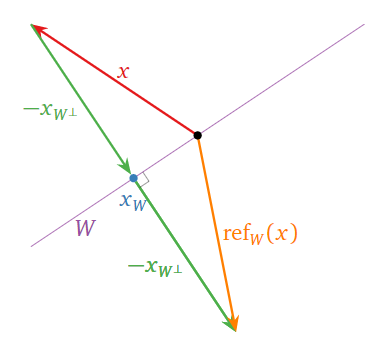
Figure \(\PageIndex{14}\)
Since \(x_{W^\perp} = x - x_W\text{,}\) we also have
\[ \text{ref}_W(x) = x - 2(x - x_W) = 2x_W - x. \nonumber \]
We leave it to the reader to check using the definition that:
- \(\text{ref}_W\circ\text{ref}_W = \text{Id}_{\mathbb{R}^n }.\)
- The \(1\)-eigenspace of \(\text{ref}_W\) is \(W\text{,}\) and the \(-1\)-eigenspace of \(\text{ref}_W\) is \(W^\perp\).
- \(\text{ref}_W\) is similar to the diagonal matrix with \(m = \dim(W)\) ones on the diagonal and \(n-m\) negative ones.