10.4: Composición de funciones

Definición: Función compuesta

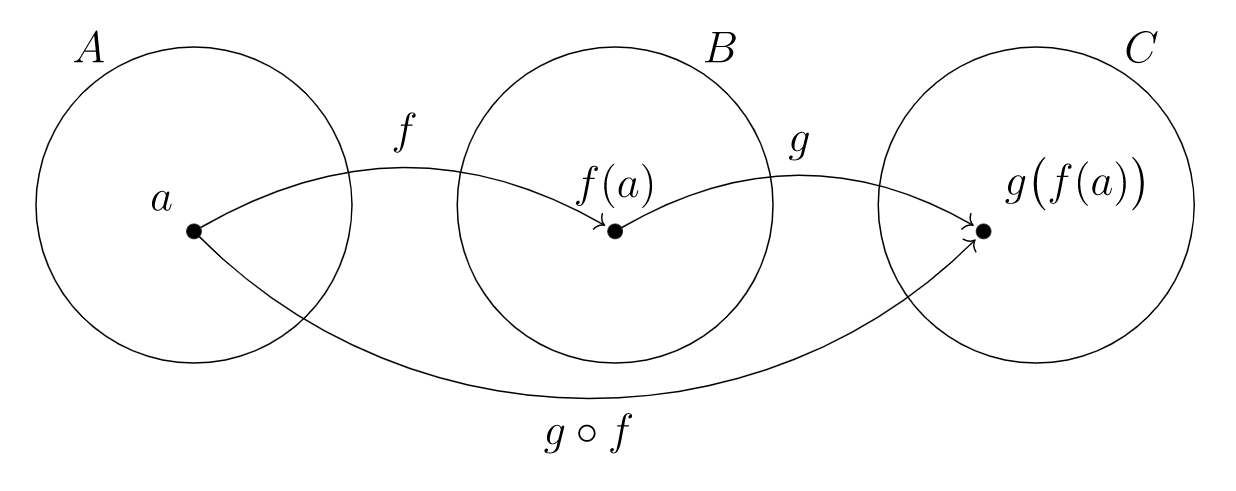
una función\(A \to C\) creada a partir de funciones dadas\(f: A \rightarrow B\) y\(g: B \rightarrow C\) por\(a \mapsto g(f(a))\)

Definición:\(g \circ f\)

la composición de las funciones\(f: A \rightarrow B\) y\(g: B \rightarrow C\text{,}\) para que\(g \circ f: A\rightarrow C\) por\((g \circ f)(a) = g(f(a))\)

Figura\(\PageIndex{1}\): Diagrama de Venn de una composición de función.

Ejemplo\(\PageIndex{1}\): A composition of two functions.

Considerar las funciones

\ begin {align*} f\ colon\ mathbb {R} &\ a\ mathbb {R} _ {\ geq 0}, & g\ colon\ mathbb {R} _ {\ geq 0} &\ a\ mathbb {R} _ _ {\ geq 0},\\ x &\ mapsto x^2, & x &\ mapsto\ sqrt {x},\ end align{ *}
Entonces tenemos

\ begin {alinear*} g\ circ f\ colon\ mathbb {R} &\ a\ mathbb {R} _ {\ geq 0},\\ x &\ mapsto\ sqrt {x^2} =\ vert x\ vert. \ end {alinear*}

Advertencia: El orden de composición importa.

La notación para la composición de funciones\(f\) e\(g\) implica una inversión de orden, así que escribimos\(g \circ f\text{.}\) Esto es para que cuando usamos esta notación con notación input-output\((g \circ f)(a)\text{,}\) la notación nos recuerda que primero se\(f\) debe aplicar a la entrada\(a\text{,}\) y luego \(g\)se aplica al resultado\(f(a)\text{.}\)

En general,\(f \circ g \ne g \circ f\text{.}\) Usualmente, uno de los dos ni siquiera está definido, porque dominios y codominios de\(f\) y\(g\) no necesariamente coincidirán en ambos órdenes. Y cuando ambos están definidos, los dos órdenes diferentes de composición suelen tener diferentes dominios y codominios.

Ejemplo\(\PageIndex{2}\): Comparing composition order.

Considerar funciones

\ begin {align*} f\ colon\ mathbb {N} &\ a\ mathbb {N}, & g\ colon\ mathbb {N} &\ a\ mathbb {N},\\ n &\ mapsto n^2, & n &\ mapsto n + 1. \ end {align*}
Entonces, ambos\(f \circ g: \mathbb{N} \rightarrow \mathbb{N}\) y\(g \circ f: \mathbb{N} \rightarrow \mathbb{N}\) se definen. Pero no son iguales, como

\ begin {alinear*} (f\ circ g) (n) & = (n+1) ^2 = n^2+2n+1, & (g\ circ f) (n) & = n^2+1. \ end {alinear*}

Ejemplo\(\PageIndex{3}\): An undefined composition.

Considerar funciones

\ begin {align*}\ text {sqrt}\ colon\ mathbb {N} &\ a\ mathbb {R}, &\ text {flr}\ colon\ mathbb {R} &\ a\ mathbb {Z},\\ n &\ mapsto\ sqrt {n}, & x &\ mapsto\ lpiso x\ rpiso. \ end {align*}
(Ver Ejemplo 10.3.4 para una descripción de la\(\text{flr}\) función.)

Entonces,\(\text{flr} \circ \text{sqrt} : \mathbb{N} \rightarrow \mathbb{Z}\) se define, con

\ begin {ecuación*} (\ text {flr}\ circ\ text {sqrt}) (n) =\ lfloor\ sqrt {n}\ rfloor\ text {.} \ end {ecuation*}
Pero no\(\text{sqrt} \circ \text{flr}\) está definido, ya que el codominio de\(\text{flr}\) no coincide con el dominio de\(\text{sqrt} \text{.}\) En particular,\(\text{flr}\) a veces devolverá una salida negativa, y no podemos usar tal salida como entrada en\(\text{sqrt} \text{.}\)

Punto de control: Propiedades de las composiciones.

Considerar funciones\(f: A \rightarrow B\) y\(g: B \rightarrow C\text{.}\)

Si\(g \circ f\) es inyectivo, ¿alguna o ambas son\(f,g\) necesariamente inyectables?

Responda la misma pregunta que la anterior con “inyectiva” reemplazada por “suryectiva”.

Demostrar que si ambos\(f\) y\(g\) son biyectivos, entonces la composición también\(g \circ f\) es biyectiva.

Por supuesto, podemos componer cualquier número de funciones.

Ejemplo\(\PageIndex{4}\): A composition of three functions.

Reconsideremos la función definida por algoritmo en el Ejemplo 10.1.3. Como la descripción de la función implicaba un algoritmo de varios pasos, deberíamos ser capaces de romper los pasos involucrados en sus propias funciones, luego recrear las funciones originales como una composición.

En primer lugar, definir\(\text{abs} : \mathscr{P}( \mathbb{Z}) \rightarrow \mathscr{P}( \mathbb{N})\) por

\ begin {ecuación*}\ texto {abs} (X) =\ {\ vert x\ vert\;\ vert x\ in X\}\ texto {.} \ end {equation*}
A continuación, defina\(min : \mathscr{P}( \mathbb{N}) \rightarrow \mathbb{N}\) para que\(\text{min}(X)\) genere el número mínimo en conjunto de entrada\(X\text{,}\) y salidas\(0\) en caso\(X = \emptyset\text{.}\)

Por último, definir\(f: \mathbb{N} \rightarrow \mathbb{N}\) por\(f(n) = 2 n + 1\text{.}\)

Cada una de estas funciones representa un paso en el algoritmo definiendo la función en el Ejemplo 10.1.3, pero para recrear esa función necesitamos componer las funciones en el orden correcto: escribir\(\varphi = f \circ \text{min} \circ \text{abs}\text{,}\) para que

\ begin {ecuation*}\ varphi (X) = 2\ text {min} (\ text {abs} (X)) + 1\ end {equation*}
calcula el mismo resultado para un conjunto\(X\) de entrada que el algoritmo descrito en el Ejemplo 10.1.3.