
8.2: Estabilidad y clasificación de puntos críticos aislados
- Page ID
- 115452

Puntos Críticos Aislados y Sistemas Casi Lineales
Un punto crítico se aísla si es el único punto crítico en algún pequeño “barrio” del punto. Es decir, si nos acercamos lo suficiente es el único punto crítico que vemos. En el ejemplo anterior, se aisló el punto crítico. Si por otro lado hubiera toda una curva de puntos críticos, entonces no estaría aislada.
Un sistema se llama casi lineal (en un punto crítico\((x_0,y_0)\)) if the critical point is isolated and the Jacobian at the point is invertible, or equivalently if the linearized system has an isolated critical point. In such a case, the nonlinear terms will be very small and the system will behave like its linearization, at least if we are close to the critical point.
En particular el sistema que acabamos de ver en los Ejemplos 8.1.1 y 8.1.2 tiene dos puntos críticos aislados\((0,0)\) and \((0,1)\), and is almost linear at both critical points as both of the Jacobian matrices \( \begin{bmatrix} 0 & 1 \\ -1 & 0 \end{bmatrix}\) and \( \begin{bmatrix} 0 & 1 \\ 1 & 0 \end{bmatrix} \) are invertible.
Por otro lado un sistema como\(x' = x^2\),\(y' = y^2\) has an isolated critical point at \((0,0)\), however the Jacobian matrix
\[\begin{bmatrix} 2x & 0 \\ 0 & 2y \end{bmatrix} \nonumber \]
es cero cuando\((x,y) = (0,0)\). Therefore the system is not almost linear. Even a worse example is the system \(x' = x\),\(y' = x^2\),which does not have an isolated critical point, as \(x'\) and \(y'\) are both zero whenever \(x=0\), that is, the entire \(y\) axis.
Afortunadamente, la mayoría de las veces los puntos críticos están aislados, y el sistema es casi lineal en los puntos críticos. Entonces, si nos enteramos de lo que sucede aquí, hemos descubierto la mayoría de las situaciones que surgen en las aplicaciones.
Estabilidad y Clasificación de Puntos Críticos Aislados
Una vez que tenemos un punto crítico aislado, el sistema es casi lineal en ese punto crítico, y calculamos el sistema linealizado asociado, podemos clasificar lo que sucede con las soluciones. Más o menos utilizamos la clasificación para sistemas lineales de dos variables de la Sección 3.5, con una advertencia menor. Listemos los comportamientos en función de los valores propios de la matriz jacobiana en el punto crítico en la Tabla\(\PageIndex{1}\). Esta tabla es muy similar a la Tabla 3.5.1, con la excepción de los puntos “centrales” faltantes. Hablaremos de los centros más adelante, ya que son más complicados.
| Valores propios de la matriz jacobiana | Comportamiento | Estabilidad |
|---|---|---|
| reales y ambos positivos | fuente/nodo inestable | inestable |
| real y ambos negativos | hundido/ nodo estable | asintóticamente estable |
| signos reales y opuestos | sillín | inestable |
| complejo con parte real positiva | fuente espiral | inestable |
| complejo con parte real negativa | fregadero espiral | asintóticamente estable |
En la nueva tercera columna, hemos marcado los puntos como asintóticamente estables o inestables. Formalmente, un punto crítico estable\((x_0,y_0)\) is one where given any small distance \(\epsilon\) to \((x_0,y_0)\),and any initial condition within a perhaps smaller radius around \((x_0,y_0)\),the trajectory of the system will never go further away from \((x_0,y_0)\) than \(\epsilon\). An unstable critical point is one that is not stable. Informally, a point is stable if we start close to a critical point and follow a trajectory we will either go towards, or at least not get away from, this critical point.
Un punto crítico estable\((x_0,y_0)\) is called asymptotically stable if given any initial condition sufficiently close to \((x_0,y_0)\) and any solution \(\bigl( x(t), y(t) \bigr)\) given that condition, then
\[\lim_{t \to \infty} \bigl( x(t), y(t) \bigr) = (x_0,y_0) . \nonumber \]
Es decir, el punto crítico es asintóticamente estable si alguna trayectoria para una condición inicial suficientemente cercana va hacia el punto crítico\((x_0,y_0)\).
Considerar\(x'=-y-x^2\), \(y'=-x+y^2\). See Figure \(\PageIndex{1}\) for the phase diagram. Let us find the critical points. These are the points where \(-y-x^2 = 0\) and \(-x+y^2=0\). The first equation means \(y = -x^2\), and so \(y^2 = x^4\). Plugging into the second equation we obtain \(-x+x^4 = 0\). Factoring we obtain \(x(1-x^3)=0\). Since we are looking only for real solutions we get either \(x=0\) or \(x=1\). Solving for the corresponding \(y\) using \(y = -x^2\),we get two critical points, one being \((0,0)\) and the other being \((1,-1)\). Clearly the critical points are isolated. Let us compute the Jacobian matrix:
\[\begin{bmatrix}-2x & -1 \\-1 & 2y\end{bmatrix} . \nonumber \]
En el punto\((0,0)\) we get the matrix \(\left[ \begin{smallmatrix} 0 & -1 \\ -1 & 0 \end{smallmatrix} \right]\) and so the two eigenvalues are \(1\) and \(-1\). As the matrix is invertible, the system is almost linear at \((0,0)\). As the eigenvalues are real and of opposite signs, we get a saddle point, which is an unstable equilibrium point.
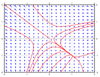
En el punto\((1,-1)\) we get the matrix \(\left[ \begin{smallmatrix} -2 & -1 \\ -1 & -2 \end{smallmatrix} \right]\) y calculando los valores propios obtenemos\(-1\),\(-3\).The matrix is invertible, and so the system is almost linear at \((1,-1)\). As we have real valores propios tanto negativos, el punto crítico es un sumidero, y por lo tanto un punto de equilibrio asintóticamente estable. Es decir, si empezamos con algún punto\((x_i,y_i)\) close to \((1,-1)\) as an initial condition and plot a trajectory, it will approach \((1,-1)\). In other words,
\[\lim_{t \to \infty} \bigl( x(t), y(t) \bigr) = (1,-1) . \nonumber \]
Como puede ver en el diagrama, este comportamiento es cierto incluso para algunos puntos iniciales bastante lejos de\((1,-1)\),but it is definitely not true for all initial points.
Echemos un vistazo a\(x'=y+y^2e^x\), \(y'=x\). First let us find the critical points. These are the points where \(y+y^2e^x = 0\) and \(x=0\). Simplifying we get \(0=y+y^2 = y(y+1)\). So the critical points are \((0,0)\) and \((0,-1)\),and hence are isolated. Let us compute the Jacobian matrix:
\[\begin{bmatrix}y^2e^x & 1+2ye^x \\1 & 0\end{bmatrix}. \nonumber \]
En el punto\((0,0)\) we get the matrix \(\left[ \begin{smallmatrix} 0 & 1 \\ 1 & 0 \end{smallmatrix} \right]\) and so the two eigenvalues are \(1\) and \(-1\). As the matrix is invertible, the system is almost linear at \((0,0)\). And, as the eigenvalues are real and of opposite signs, we get a saddle point, which is an unstable equilibrium point.
En el punto\((0,-1)\) we get the matrix \(\left[ \begin{smallmatrix} 1 & -1 \\ 1 & 0 \end{smallmatrix} \right]\) whose eigenvalues are \(\frac{1}{2} \pm i \frac{\sqrt{3}}{2}\). The matrix is invertible, and so the system is almost linear at \((0,-1)\). As we have complex eigenvalues with positive real part, the critical point is a spiral source, and therefore an unstable equilibrium point.
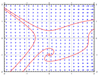
Ver Figura\(\PageIndex{2}\) para el diagrama de fases. Observe los dos puntos críticos, y el comportamiento de las flechas en el campo vectorial alrededor de estos puntos.
Problemas con los centros
Recordemos, un sistema lineal con un centro significó que las trayectorias viajaron en órbitas elípticas cerradas en alguna dirección alrededor del punto crítico. Un punto tan crítico llamaríamos un centro o un centro estable. No sería un punto crítico asintóticamente estable, ya que las trayectorias nunca se acercarían al punto crítico, pero al menos si comienzas lo suficientemente cerca del punto crítico, te quedarás cerca del punto crítico. El ejemplo más simple de tal comportamiento es el sistema lineal con un centro. Otro ejemplo es el punto crítico\((0,0)\) in Example 8.1.1.
El problema con un centro en un sistema no lineal es que si la trayectoria va hacia o lejos del punto crítico se rige por el signo de la parte real de los valores propios del jacobiano. Dado que esta parte real es cero en el punto crítico en sí mismo, puede tener cualquier señal cerca, lo que significa que la trayectoria podría ser arrastrada hacia o lejos del punto crítico.
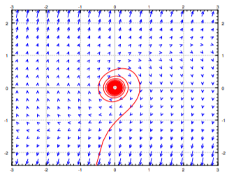
Un ejemplo fácil donde se exhibe un comportamiento tan problemático es el sistema\(x'=y, y' = -x+y^3\). The only critical point is the origin \((0,0)\). The Jacobian matrix is
\[\begin{bmatrix}0 & 1 \\-1 & 3 y^2 \\ \end{bmatrix} . \nonumber \]
En\((0,0)\) the Jacobian matrix is \(\left[ \begin{smallmatrix}0 & 1 \\-1 & 0 \\\end{smallmatrix} \right]\),which has eigenvalues \(\pm i\). Therefore, the linearization has a center.
Usando la ecuación cuadrática, los valores propios de la matriz jacobiana en cualquier punto\((x,y)\) are
\[\lambda = \frac{3}{2}y^2 \pm i \frac{\sqrt{4-9y^4}}{2} . \nonumber \]
En cualquier punto donde\(y \not= 0\) (so at most points near the origin), the eigenvalues have a positive real part (\(y^2\) can never be negative). This positive real part will pull the trajectory away from the origin. A sample trajectory for an initial condition near the origin is given in Figure \(\PageIndex{3}\).
La moraleja del ejemplo es que se necesita un mayor análisis cuando la linealización tiene un centro. El análisis será en general más complicado que en el ejemplo anterior, y es más probable que implique una consideración caso por caso. Tal complicación no debería sorprenderte. A estas alturas en tu carrera matemática, has visto muchos lugares donde una simple prueba no es concluyente, quizás comenzando con la segunda prueba derivada para máximos o mínimos, y requiere un análisis más cuidadoso, y tal vez ad hoc de la situación.
Ecuaciones Conservadoras
Una ecuación de la forma
\[x'' + f(x) = 0 \nonumber \]
para una función arbitraria\(f(x)\) is called a conservative equation. For example the pendulum equation is a conservative equation. The equations are conservative as there is no friction in the system so the energy in the system is "conserved." Let us write this equation as a system of nonlinear ODE.
\[x' = y, \qquad y' = -f(x) . \nonumber \]
Este tipo de ecuaciones tienen la ventaja de que podemos resolver por sus trayectorias fácilmente. El truco es pensar primero en\(y\) as a function of \(x\) for a moment. Then use the chain rule
\[x'' = y' = y \frac{dy}{dx} , \nonumber \]
donde el primo indica una derivada con respecto a\(t\). We obtain \(y \frac{dy}{dx} + f(x) = 0\). We integrate with respect to \(x\) to get \(\int y \frac{dy}{dx} \,dx + \int f(x)\, dx = C\). In other words
\[\frac{1}{2} y^2 + \int f(x)\, dx = C . \nonumber \]
Obtuvimos una ecuación implícita para las trayectorias, con diferentes\(C\) giving different trajectories. The value of \(C\) is conserved on any trajectory. This expression is sometimes called the Hamiltonian or the energy of the system. If you look back to Section 1.8, you will notice that \(y\frac{dy}{dx} + f(x) = 0\) is an exact equation, and we just found a potential function.
Encontremos las trayectorias para la ecuación\(x'' + x-x^2 = 0\), which is the equation from Example 8.1.1. The corresponding first order system is
\[x' = y , \qquad y' = -x+x^2 . \nonumber \]
Trayectorias satisfacen
\[\frac{1}{2} y^2 + \frac{1}{2} x^2 - \frac{1}{3} x^3 = C . \nonumber \]
Resolvemos para\(y\)
\[y = \pm \sqrt{-x^2 + \frac{2}{3} x^3 + 2C} . \nonumber \]
Trazando estas gráficas obtenemos exactamente las trayectorias en la Figura 8.1.2. En particular notamos que cerca del origen las trayectorias son curvas cerradas: siguen rodeando el origen, nunca entrando o saliendo en espiral. Por lo tanto, descubrimos una manera de verificar que el punto crítico\((0,0)\) is a stable center. The critical point at \((0,1)\) is a saddle as we already noticed. This example is typical for conservative equations.
Consideremos una ecuación conservadora arbitraria. Las trayectorias están dadas por
\[y = \pm \sqrt{ - 2 \int f(x)\, dx + 2C} . \nonumber \]
Así que todas las trayectorias se reflejan a través del\(x\)-axis. In particular, there can be no spiral sources nor sinks. All critical points occur when \(y=0\) (the \(x\)-axis), that is when \(x' = 0\). The critical points are simply those points on the \(x\)-axis where \(f(x) = 0\). The Jacobian matrix is
\[\begin{bmatrix}0 & 1 \\-f'(x) & 0\end{bmatrix} . \nonumber \]
Entonces el punto crítico es casi lineal si\(f'(x) \not= 0\) at the critical point. Let \(J\) denote the Jacobian matrix, then the eigenvalues of \(J\) are solutions to
\[0 = \det(J - \lambda I) = \lambda^2 + f'(x) . \nonumber \]
Por lo tanto\(\lambda = \pm \sqrt{-f'(x)}\). In other words, either we get real eigenvalues of opposite signs, or we get purely imaginary eigenvalues. There are only two possibilities for critical points, either an unstable saddle point, or a stable center. There are never any asymptotically stable points, sinks, or sources.