
4.7: Función Gamma
- Page ID
- 119589

Una función que a menudo ocurre en el estudio de las funciones especiales es la función Gamma. Necesitaremos la función Gamma en la siguiente sección sobre la serie Fourier-Bessel.
Porque\(x>0\) definimos la función Gamma como
\[\Gamma(x)=\int_{0}^{\infty} t^{x-1} e^{-t} d t, \quad x>0 \nonumber \]
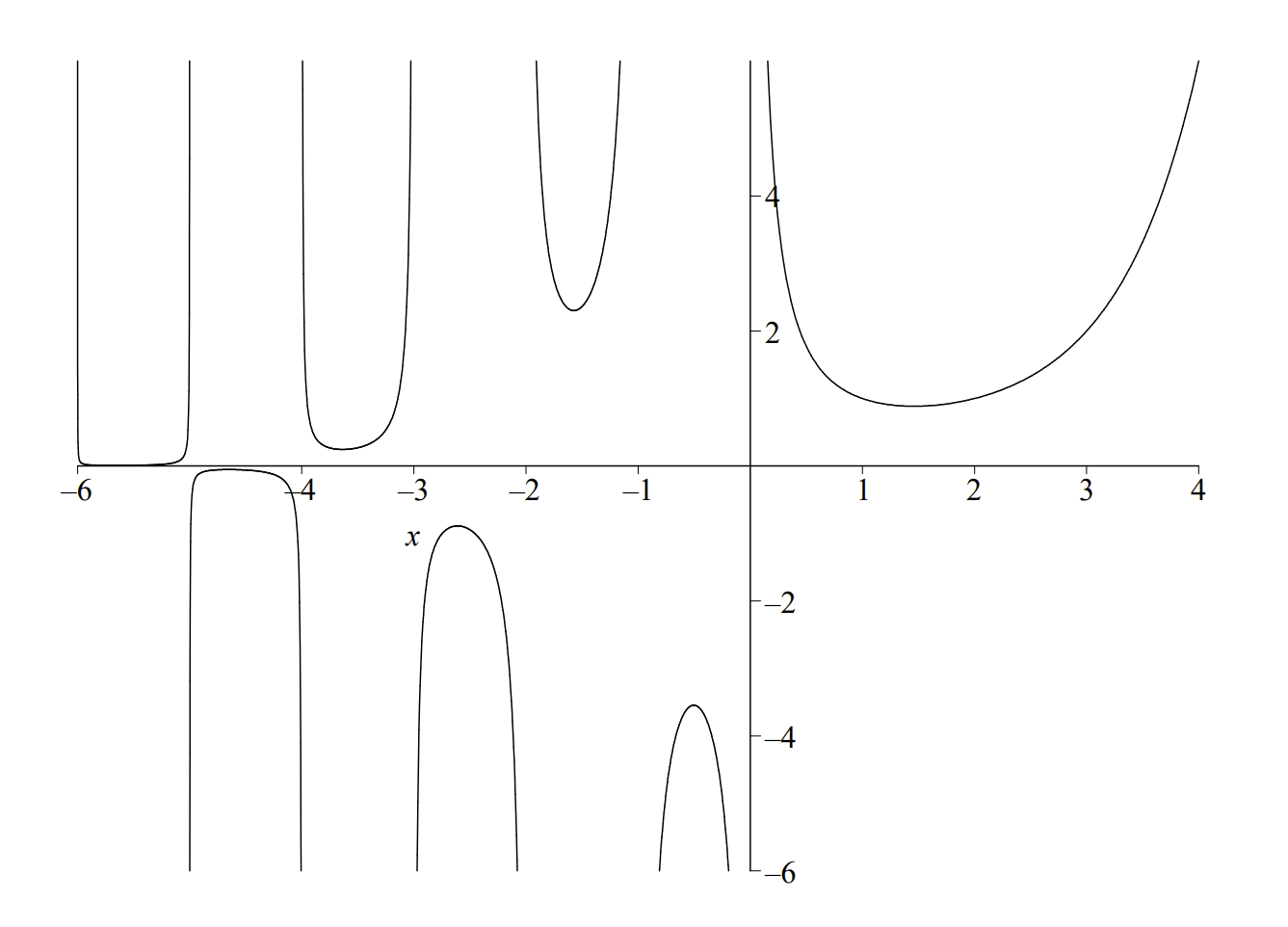
El nombre y el símbolo de la función Gamma fueron dados por primera vez por Legendre en 1811. Sin embargo, la búsqueda de una generalización de lo factorial se remonta a\(1720^{\prime} \mathrm{s}\) cuando Euler proporcionó la primera representación del factorial como un producto infinito, posteriormente para ser modificado por otros como Gauß, Weierstraß y Legendre. La función Gamma es una generalización de la función factorial y se muestra una gráfica en la Figura\(4.5\). De hecho, tenemos
\[\Gamma(1)=1 \nonumber \]
y
\[\Gamma(x+1)=x \Gamma(x) \nonumber \]
El lector puede probar esta identidad simplemente realizando una integración por partes. (Ver Problema 13.) En particular, para los enteros\(n \in Z^{+}\), tenemos entonces
\[\Gamma(n+1)=n \Gamma(n)=n(n-1) \Gamma(n-2)=n(n-1) \cdots 2 \Gamma(1)=n ! \nonumber \]
También podemos definir la función Gamma para valores negativos, no enteros de Primero\(x .\) notamos que por iteración en\(n \in Z^{+}\), tenemos
\[\Gamma(x+n)=(x+n-1) \cdots(x+1) x \Gamma(x), \quad x+n>0 \nonumber \]
Resolviendo para\(\Gamma(x)\), luego encontramos
\[\Gamma(x)=\dfrac{\Gamma(x+n)}{(x+n-1) \cdots(x+1) x}, \quad-n<x<0 \nonumber \]
Tenga en cuenta que la función Gamma no está definida en cero y los enteros negativos.
Ahora demostramos que
\[\Gamma\left(\dfrac{1}{2}\right)=\sqrt{\pi}. \nonumber \]
Esto se hace por cómputo directo de la integral:
\[\Gamma\left(\dfrac{1}{2}\right)=\int_{0}^{\infty} t^{-\dfrac{1}{2}} e^{-t} d t \nonumber \]
Dejando\(t=z^{2}\), tenemos
\[\Gamma\left(\dfrac{1}{2}\right)=2 \int_{0}^{\infty} e^{-z^{2}} d z\nonumber \]
Debido a la simetría del integrando, obtenemos el clásico inte-
\({ }^{4}\)Usando una sustitución\(x^{2}=\beta y^{2}\), podemos mostrar gral4 el resultado más general:
\[\Gamma\left(\dfrac{1}{2}\right)=\int_{-\infty}^{\infty} e^{-z^{2}} d z,\nonumber \]
\[\int_{-\infty}^{\infty} e^{-\beta y^{2}} d y=\sqrt{\dfrac{\pi}{\beta}}\nonumber \]
Que se puede realizar usando un truco estándar. Considera lo integral.
\[I=\int_{-\infty}^{\infty} e^{-x^{2}} d x\nonumber \]
Entonces,
\[I^{2}=\int_{-\infty}^{\infty} e^{-x^{2}} d x \int_{-\infty}^{\infty} e^{-y^{2}} d y\nonumber \]
Tenga en cuenta que cambiamos la variable de integración. Esto escribe este producto de integrales como una doble integral:
\[I^{2}=\int_{-\infty}^{\infty} \int_{-\infty}^{\infty} e^{-\left(x^{2}+y^{2}\right)} d x d y \nonumber \]
Tenga en cuenta que cambiamos la variable de integración. Esto nos permitirá Esto es una integral sobre todo el\(x y\) -plano. Podemos transformar esta integración cartesiana en una integración sobre coordenadas polares. La integral se convierte en
\[I^{2}=\int_{0}^{2 \pi} \int_{0}^{\infty} e^{-r^{2}} r d r d \theta \nonumber \]
Esto es sencillo de integrar y tenemos\(I^{2}=\pi .\) Así, el resultado final se encuentra tomando la raíz cuadrada de ambos lados:
\[\Gamma\left(\dfrac{1}{2}\right)=I=\sqrt{\pi} \nonumber \]
En Problema 15, el lector demostrará la identidad más general
\[\Gamma\left(n+\dfrac{1}{2}\right)=\dfrac{(2 n-1) ! !}{2^{n}} \sqrt{\pi} \nonumber \]
Otra relación útil, que sólo declaramos, es
\[\Gamma(x) \Gamma(1-x)=\dfrac{\pi}{\sin \pi x} \nonumber \]
Son muchas otras relaciones importantes, entre ellas productos infinitos, que no necesitaremos en este momento. Se anima al lector a leer sobre estos en otra parte. Mientras tanto, pasamos a la discusión de otra función especial importante en física y matemáticas.