Saltar al contenido principal
LibreTexts Español

7.6: Método de coordenadas

  • Page ID
    114398
  • \( \newcommand{\vecs}[1]{\overset { \scriptstyle \rightharpoonup} {\mathbf{#1}} } \)

    \( \newcommand{\vecd}[1]{\overset{-\!-\!\rightharpoonup}{\vphantom{a}\smash {#1}}} \)

    \( \newcommand{\id}{\mathrm{id}}\) \( \newcommand{\Span}{\mathrm{span}}\)

    ( \newcommand{\kernel}{\mathrm{null}\,}\) \( \newcommand{\range}{\mathrm{range}\,}\)

    \( \newcommand{\RealPart}{\mathrm{Re}}\) \( \newcommand{\ImaginaryPart}{\mathrm{Im}}\)

    \( \newcommand{\Argument}{\mathrm{Arg}}\) \( \newcommand{\norm}[1]{\| #1 \|}\)

    \( \newcommand{\inner}[2]{\langle #1, #2 \rangle}\)

    \( \newcommand{\Span}{\mathrm{span}}\)

    \( \newcommand{\id}{\mathrm{id}}\)

    \( \newcommand{\Span}{\mathrm{span}}\)

    \( \newcommand{\kernel}{\mathrm{null}\,}\)

    \( \newcommand{\range}{\mathrm{range}\,}\)

    \( \newcommand{\RealPart}{\mathrm{Re}}\)

    \( \newcommand{\ImaginaryPart}{\mathrm{Im}}\)

    \( \newcommand{\Argument}{\mathrm{Arg}}\)

    \( \newcommand{\norm}[1]{\| #1 \|}\)

    \( \newcommand{\inner}[2]{\langle #1, #2 \rangle}\)

    \( \newcommand{\Span}{\mathrm{span}}\) \( \newcommand{\AA}{\unicode[.8,0]{x212B}}\)

    \( \newcommand{\vectorA}[1]{\vec{#1}}      % arrow\)

    \( \newcommand{\vectorAt}[1]{\vec{\text{#1}}}      % arrow\)

    \( \newcommand{\vectorB}[1]{\overset { \scriptstyle \rightharpoonup} {\mathbf{#1}} } \)

    \( \newcommand{\vectorC}[1]{\textbf{#1}} \)

    \( \newcommand{\vectorD}[1]{\overrightarrow{#1}} \)

    \( \newcommand{\vectorDt}[1]{\overrightarrow{\text{#1}}} \)

    \( \newcommand{\vectE}[1]{\overset{-\!-\!\rightharpoonup}{\vphantom{a}\smash{\mathbf {#1}}}} \)

    \( \newcommand{\vecs}[1]{\overset { \scriptstyle \rightharpoonup} {\mathbf{#1}} } \)

    \( \newcommand{\vecd}[1]{\overset{-\!-\!\rightharpoonup}{\vphantom{a}\smash {#1}}} \)

    \(\newcommand{\avec}{\mathbf a}\) \(\newcommand{\bvec}{\mathbf b}\) \(\newcommand{\cvec}{\mathbf c}\) \(\newcommand{\dvec}{\mathbf d}\) \(\newcommand{\dtil}{\widetilde{\mathbf d}}\) \(\newcommand{\evec}{\mathbf e}\) \(\newcommand{\fvec}{\mathbf f}\) \(\newcommand{\nvec}{\mathbf n}\) \(\newcommand{\pvec}{\mathbf p}\) \(\newcommand{\qvec}{\mathbf q}\) \(\newcommand{\svec}{\mathbf s}\) \(\newcommand{\tvec}{\mathbf t}\) \(\newcommand{\uvec}{\mathbf u}\) \(\newcommand{\vvec}{\mathbf v}\) \(\newcommand{\wvec}{\mathbf w}\) \(\newcommand{\xvec}{\mathbf x}\) \(\newcommand{\yvec}{\mathbf y}\) \(\newcommand{\zvec}{\mathbf z}\) \(\newcommand{\rvec}{\mathbf r}\) \(\newcommand{\mvec}{\mathbf m}\) \(\newcommand{\zerovec}{\mathbf 0}\) \(\newcommand{\onevec}{\mathbf 1}\) \(\newcommand{\real}{\mathbb R}\) \(\newcommand{\twovec}[2]{\left[\begin{array}{r}#1 \\ #2 \end{array}\right]}\) \(\newcommand{\ctwovec}[2]{\left[\begin{array}{c}#1 \\ #2 \end{array}\right]}\) \(\newcommand{\threevec}[3]{\left[\begin{array}{r}#1 \\ #2 \\ #3 \end{array}\right]}\) \(\newcommand{\cthreevec}[3]{\left[\begin{array}{c}#1 \\ #2 \\ #3 \end{array}\right]}\) \(\newcommand{\fourvec}[4]{\left[\begin{array}{r}#1 \\ #2 \\ #3 \\ #4 \end{array}\right]}\) \(\newcommand{\cfourvec}[4]{\left[\begin{array}{c}#1 \\ #2 \\ #3 \\ #4 \end{array}\right]}\) \(\newcommand{\fivevec}[5]{\left[\begin{array}{r}#1 \\ #2 \\ #3 \\ #4 \\ #5 \\ \end{array}\right]}\) \(\newcommand{\cfivevec}[5]{\left[\begin{array}{c}#1 \\ #2 \\ #3 \\ #4 \\ #5 \\ \end{array}\right]}\) \(\newcommand{\mattwo}[4]{\left[\begin{array}{rr}#1 \amp #2 \\ #3 \amp #4 \\ \end{array}\right]}\) \(\newcommand{\laspan}[1]{\text{Span}\{#1\}}\) \(\newcommand{\bcal}{\cal B}\) \(\newcommand{\ccal}{\cal C}\) \(\newcommand{\scal}{\cal S}\) \(\newcommand{\wcal}{\cal W}\) \(\newcommand{\ecal}{\cal E}\) \(\newcommand{\coords}[2]{\left\{#1\right\}_{#2}}\) \(\newcommand{\gray}[1]{\color{gray}{#1}}\) \(\newcommand{\lgray}[1]{\color{lightgray}{#1}}\) \(\newcommand{\rank}{\operatorname{rank}}\) \(\newcommand{\row}{\text{Row}}\) \(\newcommand{\col}{\text{Col}}\) \(\renewcommand{\row}{\text{Row}}\) \(\newcommand{\nul}{\text{Nul}}\) \(\newcommand{\var}{\text{Var}}\) \(\newcommand{\corr}{\text{corr}}\) \(\newcommand{\len}[1]{\left|#1\right|}\) \(\newcommand{\bbar}{\overline{\bvec}}\) \(\newcommand{\bhat}{\widehat{\bvec}}\) \(\newcommand{\bperp}{\bvec^\perp}\) \(\newcommand{\xhat}{\widehat{\xvec}}\) \(\newcommand{\vhat}{\widehat{\vvec}}\) \(\newcommand{\uhat}{\widehat{\uvec}}\) \(\newcommand{\what}{\widehat{\wvec}}\) \(\newcommand{\Sighat}{\widehat{\Sigma}}\) \(\newcommand{\lt}{<}\) \(\newcommand{\gt}{>}\) \(\newcommand{\amp}{&}\) \(\definecolor{fillinmathshade}{gray}{0.9}\)

    El siguiente ejercicio es importante; demuestra que nuestra definición axiomática concuerda con la definición del modelo.

    Ejercicio\(\PageIndex{1}\)

    2021-02-11 11.29.32.png

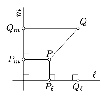
    Dejar\(\ell\) y\(m\) ser líneas perpendiculares en el plano euclidiano. Dado un punto\(P\), vamos\(P_{\ell}\) y\(P_m\) denotan los puntos del pie de\(P\) on\(\ell\) y\(m\) respectivamente.

    1. Demostrar que para cualquier\(X \in \ell\) y\(Y \in m\) hay un punto único\(P\) tal que\(P_{\ell} = X\) y\(P_m = Y\).
    2. Demuestre eso\(PQ^2 = P_{\ell}Q_{\ell}^2 + P_m Q_m^2\) para cualquier par de puntos\(P\) y\(Q\).
    3. Concluir que el plano es isométrico a\((\mathbb{R}^2, d_2)\).
    Pista

    (a). Utilizar la singularidad de la línea paralela (Teorema 7.1.1).

    b). Usa Lema 7.5.1 y el teorema de Pitágoras (Teorema 6.2.1)

    Una vez resuelto este ejercicio, podemos aplicar el método de coordenadas para resolver cualquier problema en la geometría del plano euclidiano. Este método es poderoso y universal; se desarrollará más en el Capítulo 18.

    Ejercicio\(\PageIndex{2}\)

    Utilizar el Ejercicio\(\PageIndex{1}\) para dar una prueba alternativa del Teorema 3.5.1 en el plano euclídeo.

    Es decir, probar que dados los números reales\(a, b\), y\(c\) tal que

    \(0 < a \le b \le c \le a + b\),

    hay un triángulo\(ABC\) tal que\(a = BC\),\(b = CA\), y\(c = AB\).

    Pista

    Establecer\(A = (0, 0), B = (c, 0)\), y\(C = (x, y)\). Claramente,\(AB = c\),\(AC^2 = x^2 + y^2\) y\(BC^2 = (c - x)^2 + y^2\).

    Queda por demostrar que existe un par de números reales\((x, y)\) que satisfagan el siguiente sistema de ecuaciones:

    \(\begin{cases} b^2 = x^2 + y^2 \\ a^2 = (c- x)^2 + y^2 \end{cases}\)

    si\(0 < a \le b \le c \le a + c\).

    Ejercicio\(\PageIndex{3}\)

    Considera dos puntos distintos\(A = (x_A, y_A)\) y\(B = (x_B, y_B)\) en el plano de coordenadas. Mostrar que la bisectriz perpendicular a\([AB]\) es descrita por la ecuación

    \(2 \cdot (x_B - x_A) \cdot x + 2 \cdot (y_B - y_A) \cdot y = x_B^2 + y_B^2 - x_A^2 - y_B^2\).

    Concluye que la línea se puede definir como un subconjunto del plano de coordenadas del siguiente tipo:

    1. Soluciones de una ecuación\(a \cdot x + b \cdot y = c\) para algunas constantes\(a, b\), y\(c\) tal que\(a \ne 0\) o\(b \ne 0\).
    2. El conjunto de puntos\((a \cdot t + c, b \cdot t + d)\) para algunas constantes\(a, b, c\), y\(d\) tal que\(a \ne 0\) o\(b \ne 0\) y todos\(t \in \mathbb{R}\).
    Pista

    Tenga en cuenta que\(MA = MB\) si y solo si

    \((x - x_A)^2 + (y - y_A)^2 = (x - x_B)^2 + (y - y_B)^2\)

    donde\(M = (x, y)\). Para probar la primera parte, simplificar esta ecuación. Para las piezas restantes, use que cualquier línea sea una bisectriz perpendicular a algún segmento de línea.


    This page titled 7.6: Método de coordenadas is shared under a CC BY-SA 4.0 license and was authored, remixed, and/or curated by Anton Petrunin via source content that was edited to the style and standards of the LibreTexts platform.