
6.1: Resolver ecuaciones trigonométricas
- Page ID
- 113552

Una ecuación que involucra funciones trigonométricas se denomina ecuación trigonométrica. Por ejemplo, una ecuación como
\ [\ tan\; A ~=~ 0.75 ~,
\ nonumber\]
que encontramos en el Capítulo 1, es una ecuación trigonométrica. En el Capítulo 1 nos preocupaba sólo encontrar una única solución (digamos, entre\(0^\circ \) y\(90^\circ\)). En esta sección nos ocuparemos de encontrar la solución más general a tales ecuaciones.
Para ver lo que eso significa, toma la ecuación anterior\(\tan\;A = 0.75 \). Usando el botón de calculadora\(\fbox{\(\tan^{-1}\)}\) en modo grados, obtenemos\(A=36.87^\circ \). Sin embargo, sabemos que la función tangente tiene\(\pi \) rad de período\(= 180^\circ \), es decir, repite cada\(180^\circ \). Así, hay muchas otras posibles respuestas por el valor de\(A \), es decir\(36.87^\circ + 180^\circ \)\(36.87^\circ - 180^\circ \),\(36.87^\circ + 360^\circ \),\(36.87^\circ - 360^\circ \),\(36.87^\circ + 540^\circ \),, etc. Podemos escribir esto de una forma más compacta:
\ [A ~=~ 36.87^\ circ\; +\; 180^\ circ k\ quad\ texto {para\(k=0 \),\(\pm\,1 \),\(\pm\,2 \),\(...\)}
\ nonumber\]
Esta es la solución más general a la ecuación. A menudo se omite la parte que dice “for\(k=0 \)\(\pm\,1 \)\(\pm\,2 \),,\(...\)” ya que generalmente se entiende que\(k \) varía sobre todos los enteros. La solución general en radianes sería:
\ [A ~=~ 0.6435\; +\;\ pi k\ quad\ texto {para\(k=0 \),\(\pm\,1 \),\(\pm\,2 \),\(...\)}
\ nonúmero\]
Resuelve la ecuación\(\;2\,\sin\;\theta \;+\;1 ~=~ 0 \).
Solución:
Aislar\(\sin\;\theta \) da\(\;\sin\;\theta ~=~ -\tfrac{1}{2} \). El uso del botón de calculadora\(\fbox{\(\sin^{-1}\)}\) en modo grados nos da\(\theta = -30^\circ \), que está en QIV. Recordemos que la reflexión de este ángulo alrededor del\(y\) eje -eje hacia QIII también tiene el mismo seno. Es decir,\(\sin\;210^\circ = -\tfrac{1}{2} \). Así, dado que la función sinusoidal tiene período\(2\pi \) rad\(= 360^\circ \), y dado que\(-30^\circ \) no difiere de\(210^\circ \) por un múltiplo entero de\(360^\circ \), la solución general es:
\ [\ en caja {\ theta ~=~ -30^\ circ\; +\; 360^\ circ k\ quad\ texto {y}\ quad 210^\ circ\; +\;
360^\ circ k}\ qquad\ texto {para\(k=0 \),\(\pm\,1 \),\(\pm\,2 \),\(...\)}
\ nonumber\]
En radianes, la solución es:
\ [\ en caja {\ theta ~=~ -\ dfrac {\ pi} {6}\; +\; 2\ pi k\ quad\ texto {y}\ quad\ dfrac {7\ pi} {6} + 2\ pi k}
\ qquad\ texto {para\(k=0 \),\(\pm\,1 \),\(\pm\,2 \),\(...\)}
\ nonumber\]
Para el resto de esta sección escribiremos nuestras soluciones en radianes.
Resuelve la ecuación\(\;2\cos^2 \;\theta \;-\; 1 ~=~ 0 \).
Solución:
Aislar nos\(\;\cos^2 \;\theta \) da
\ [\ cos^2\;\ theta ~=~\ frac {1} {2}\ quad\ Rightarrow\ quad\ cos\;\ theta ~=~\ pm\,\ frac {1} {\ sqrt {2}}
\ quad\ Rightarrow\ quad\ theta ~=~\ frac {\ pi} {4}\;, ~\ frac {3\ pi} {4}\;, ~\ frac {5\ pi} {4}\;, ~
\ frac {7\ pi} {4} ~,
\ nonumber\]
y como el periodo del coseno es\(2\pi \), añadiríamos\(2\pi k \) a cada uno de esos ángulos para obtener la solución general. Pero fíjese que los ángulos anteriores difieren en múltiplos de\(\frac{\pi}{2} \). Entonces, dado que cada múltiplo de también\(2\pi \) es un múltiplo de\(\frac{\pi}{2} \), podemos combinar esas cuatro respuestas separadas en una sola:
\ [\ en caja {\ theta ~=~\ frac {\ pi} {4}\; +\;\ frac {\ pi} {2}\, k}
\ qquad\ texto {for\(k=0 \),\(\pm\,1 \),\(\pm\,2 \),\(...\)}
\ nonumber\]
Resuelve la ecuación\(\;2\,\sec\;\theta ~=~ 1 \).
Solución:
Aislar nos\(\;\sec\;\theta \) da
\ [\ seg\;\ theta ~=~\ frac {1} {2}\ quad\ Rightarrow\ quad\ cos\;\ theta ~=~\ frac {1} {\ sec\;\ theta} ~=~ 2~,
\ nonumber\]
lo cual es imposible. Así, la hay\(\fbox{no solution}\).
Resuelve la ecuación\(\;\cos\;\theta ~=~ \tan\;\theta \).
Solución:
La idea aquí es usar identidades para poner todo en términos de una sola función trigonométrica:
\ [\ nonumber\ begin {alinear*}
\ cos\;\ theta ~&=~\ tan\;\ theta\\\ nonumber
\ cos\;\ theta ~&=~\ frac {\ sin\;\ theta} {\ cos\;\ theta}\\ noumber
\ cos^2\;\ theta ~&=~\ sin\;\ theta\\\ nonumber
1\; -\;\ sin^2\;\ theta ~&=~\ sin\;\ theta\\\ nonumber
0 ~&=~\ sin^2\;\ theta\; +\;\ sin\;\ theta\; -\; 1
\ end {align*}\ nonumber\]
La última ecuación parece más complicada que la ecuación original, pero fíjense que en realidad es una ecuación cuadrática: haciendo la sustitución\(x=\sin\;\theta \), tenemos
\ [x^2\; +\; x\; -\; 1 ~=~ 0\ quad\ Rightarrow\ quad x ~=~\ frac {-1\;\ pm\;\ sqrt {1 - (4)\, (-1)}} {
2\, (1)} ~=~\ frac {-1\;\ pm\;\ sqrt {5}} {2} ~ -1.618\;, ~0.618
\ nonumber\]
por la fórmula cuadrática del álgebra elemental. Pero\(-1.618 < -1 \), entonces es imposible eso\(\;\sin\theta = x = -1.618 \). Por lo tanto, debemos tener\(\;\sin\;\theta = x = 0.618 \). De ahí que existan dos soluciones posibles:\(\theta = 0.666 \) rad en QI y su\(\pi - \theta = 2.475\) rad de reflexión alrededor del\(y\) eje en QII. Agregar múltiplos\(2\pi \) de estos nos da la solución general:
\ [\ en caja {\ theta ~=~ 0.666\; +\; 2\ pi k\ quad\ texto {y}\ quad 2.475\; +\; 2\ pi k}
\ qquad\ texto {para\(k=0 \),\(\pm\,1 \),\(\pm\,2 \),\(...\)}
\ nonumber\]
Resuelve la ecuación\(\;\sin\;\theta ~=~ \tan\;\theta \).
Solución:
Probando el mismo método que en el ejemplo anterior, obtenemos
\ [\ nonumber\ begin {align*}
\ sin\;\ theta ~&=~\ tan\;\ theta\\\ nonumber
\ sin\;\ theta ~&=~\ frac {\ sin\;\ theta} {\ cos\;\ theta}\\ theta}\\ nonumber
\ sin\;\ theta~\ cos\;\ theta ~&=~\ sin\;\ theta\\\ nonumber
\ sin\;\ theta~\ cos\;\ theta\; -\;\ sin\;\ theta ~&= ~ 0\\\ nonumber
\ sin\;\ theta~ (\ cos\;\ theta\; -\; 1) ~&=~ 0\\\ nonumber
&\ Rightarrow\ quad\ sin\;\ theta ~=~ 0\ quad\ text {o}\ quad\ cos\;\ theta ~=~ 1\\ nonumber
&\ Rightarrow\\ theta ~=~ 0\;, ~\ pi\ quad\ texto {o}\ quad\ theta ~=~ 0\\\ nonúmero
&\ Rightarrow\ quad\ theta ~=~ 0\;, ~\ pi~,
\ end {align*}\ nonumber\]
más múltiplos de\(2\pi \). Entonces, dado que los ángulos anteriores son múltiplos de\(\pi \), y cada múltiplo de\(2\pi \) es un múltiplo de\(\pi \), podemos combinar las dos respuestas en una sola para la solución general:
\ [\ en caja {\ theta ~=~\ pi k}\ qquad\ texto {para\(k=0 \),\(\pm\,1 \),\(\pm\,2 \),\(...\)}
\ nonumber\]
Resuelve la ecuación\(\;\cos\;3\theta ~=~ \frac{1}{2} \).
Solución:
La idea aquí es resolver por\(3\theta \) primera vez, usando la solución más general, y luego dividir esa solución por\(3 \). Entonces ya\(\;\cos^{-1} \frac{1}{2} = \frac{\pi}{3} \), hay dos posibles soluciones para\(3\theta\):\(3\theta = \frac{\pi}{3} \) en QI y su reflexión\(-3\theta = -\frac{\pi}{3} \) alrededor del\(x\) eje en QIV. Agregar múltiplos de\(2\pi \) a estos nos da:
\ [3\ theta ~=~\ pm\,\ frac {\ pi} {3}\; +\; 2\ pi k\ qquad\ texto {para\(k=0 \),\(\pm\,1 \),\(\pm\,2 \),\(...\)}
\ nonumber\]
Entonces dividiendo todo por\(3 \) obtenemos la solución general para\(\theta\):
\ [\ en caja {\ theta ~=~\ pm\,\ frac {\ pi} {9}\; +\;\ frac {2\ pi} {3} k}
\ qquad\ texto {para\(k=0 \),\(\pm\,1 \),\(\pm\,2 \),\(...\)}
\ nonumber\]
Resuelve la ecuación\(\;\sin\;2\theta ~=~ \sin\;\theta \).
Solución:
Aquí usamos la fórmula de doble ángulo para seno:
\ [\ nonumber\ begin {alinear*}
\ sin\; 2\ theta ~&=~\ sin\;\ theta\\ nonumber
2\,\ sin\ theta~\ cos\;\ theta ~&=~\ sin\;\ theta\\ nonumber
\ sin\;\ theta~ (2\,\ cos\;\ theta\; -\; 1) ~&=~ 0\\\ nonumber
&\ Rightarrow\ quad\ sin\;\ theta ~=~ 0\ quad\ texto {o}\ quad\ cos\;\ theta ~=~\ frac {1} {2}\\\ nonumber
&\ Rightarrow\ quad\ theta ~=~ 0\;, ~\ pi\ quad\ texto {o}\ quad\ theta ~=~\ pm\,\ frac {\ pi} {3}\\\ nonumber
&\ Rightarrow\ quad\ en caja {\ ththeta ~=~\ pi k\ quad\ texto {y}\ quad\ pm\,\ frac {\ pi} {3}\; +\; 2\ pi k}
\ qquad\ texto {para \(k=0 \),\(\pm\,1 \),\(\pm\,2 \),\(...\)}
\ end {align*}
\ nonumber\]
Resuelve la ecuación\(\;2\,\sin\;\theta \;-\; 3\,\cos\;\theta ~=~ 1 \).
Solución
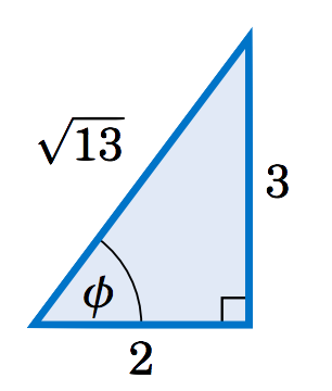
Utilizaremos la técnica que discutimos en el Capítulo 5 para encontrar la amplitud de una combinación de funciones sinusoidales y cosenales. Tomar los coeficientes\(2 \) y\(3 \) de\(\;\sin\;\theta \) y\(\;-\cos\;\theta \), respectivamente, en la ecuación anterior y hacerlos las patas de un triángulo rectángulo, como en la Figura 6.1.1. Dejar\(\phi \) ser el ángulo que se muestra en el triángulo rectángulo. La pata con longitud\(3 >0 \) significa que el ángulo\(\phi \) está por encima del\(x\) eje, y la pata con longitud\(2>0 \) significa que\(\phi \) está a la derecha del\(y\) eje. De ahí,\(\phi \) debe estar en QI. La hipotenusa tiene longitud\(\sqrt{13} \) según el Teorema de Pitágoras, y por lo tanto\(\;\cos\;\phi = \frac{2}{\sqrt{13}} \) y\(\;\sin\;\theta = \frac{3}{\sqrt{13}} \). Podemos usar esto para transformar la ecuación para resolver de la siguiente manera:
\ [\ nonumber\ begin {align*}
2\,\ sin\;\ theta\; -\; 3\,\ cos\;\ theta ~&=~ 1\\\ nonumber
\ sqrt {13}\,\ izquierda (\ tfrac {2} {\ sqrt {13}}\,\ sin\;\ theta\; -\ tfrac {3} {\ sqrt {13}}\,\ cos\;\ theta
\ derecha) ~&=~ 1\\\ nonumber
\ sqrt {13}\, (\ cos\;\ phi\;\ sin\;\ theta\; - \;\ sin\;\ phi\;\ cos\;\ theta) ~&=~ 1\\\ nonumber
\ sqrt {13}\,\ sin\ ;(\ theta -\ phi) ~&=~ 1\ quad\ text {(por la fórmula de resta sinusoidal)}\\\ nonumber
\ sin\ ;(\ theta -\ phi) ~&=~\ tfrac {1} {\ sqrt {13}}\\\ nonumber
&\ Rightarrow\ quad\ theta -\ phi ~=~ 0.281\ quad \ texto {o}\ quad\ theta -\ phi ~=~\ pi - 0.281 = 2.861\\\ nonumber
&\ Rightarrow\ quad\ theta ~=~\ phi\; +\; 0.281\ quad\ text {o}\ quad\ theta ~=~\ phi\; +\; 2.861
\ end {align*}\ nonumber\]
Ahora, ya que\(\;\cos\;\phi = \frac{2}{\sqrt{13}} \) y\(\phi \) está en QI, la solución más general para\(\phi \) es\(\phi = 0.983 + 2\pi k \) para\(k=0 \),\(\pm\,1 \),\(\pm\,2 \),\(... \). Entonces como necesitábamos agregar múltiplos de\(2\pi \) a las soluciones\(0.281 \) y de\(2.861 \) todos modos, la solución más general para\(\theta \) es:
\ [\ begin {alinear*}
\ theta ~&=~ 0.983\; +\; 0.281\; +\; 2\ pi k\ quad\ texto {y}\ quad 0.983\; +\; 2.861\; +\; 2\ pi k\
&\ Rightarrow\ quad\ boxed {\ theta ~=~ 1.264\; +\; 2\ pi k\ texto {y}\ quad 3.844\; +\; 2\ pi k}
\ cuádruple\ texto {para\(k=0 \),\(\pm\,1 \),\(\pm\,2 \), \(...\)}
\ end {align*}\ nonumber\]
Nota: En el Ejemplo 6.8 si la ecuación hubiera sido\(\;2\,\sin\;\theta \;+\; 3\,\cos\;\theta ~=~ 1 \) entonces todavía habríamos usado un triángulo rectángulo con patas de longitudes\(2 \) y\(3 \), pero habríamos usado la fórmula de suma sinusoidal en lugar de la fórmula de resta.