4.5: Significado Geométrico de la Multiplicación Escalar
- Page ID
- 114523
\( \newcommand{\vecs}[1]{\overset { \scriptstyle \rightharpoonup} {\mathbf{#1}} } \)
\( \newcommand{\vecd}[1]{\overset{-\!-\!\rightharpoonup}{\vphantom{a}\smash {#1}}} \)
\( \newcommand{\id}{\mathrm{id}}\) \( \newcommand{\Span}{\mathrm{span}}\)
( \newcommand{\kernel}{\mathrm{null}\,}\) \( \newcommand{\range}{\mathrm{range}\,}\)
\( \newcommand{\RealPart}{\mathrm{Re}}\) \( \newcommand{\ImaginaryPart}{\mathrm{Im}}\)
\( \newcommand{\Argument}{\mathrm{Arg}}\) \( \newcommand{\norm}[1]{\| #1 \|}\)
\( \newcommand{\inner}[2]{\langle #1, #2 \rangle}\)
\( \newcommand{\Span}{\mathrm{span}}\)
\( \newcommand{\id}{\mathrm{id}}\)
\( \newcommand{\Span}{\mathrm{span}}\)
\( \newcommand{\kernel}{\mathrm{null}\,}\)
\( \newcommand{\range}{\mathrm{range}\,}\)
\( \newcommand{\RealPart}{\mathrm{Re}}\)
\( \newcommand{\ImaginaryPart}{\mathrm{Im}}\)
\( \newcommand{\Argument}{\mathrm{Arg}}\)
\( \newcommand{\norm}[1]{\| #1 \|}\)
\( \newcommand{\inner}[2]{\langle #1, #2 \rangle}\)
\( \newcommand{\Span}{\mathrm{span}}\) \( \newcommand{\AA}{\unicode[.8,0]{x212B}}\)
\( \newcommand{\vectorA}[1]{\vec{#1}} % arrow\)
\( \newcommand{\vectorAt}[1]{\vec{\text{#1}}} % arrow\)
\( \newcommand{\vectorB}[1]{\overset { \scriptstyle \rightharpoonup} {\mathbf{#1}} } \)
\( \newcommand{\vectorC}[1]{\textbf{#1}} \)
\( \newcommand{\vectorD}[1]{\overrightarrow{#1}} \)
\( \newcommand{\vectorDt}[1]{\overrightarrow{\text{#1}}} \)
\( \newcommand{\vectE}[1]{\overset{-\!-\!\rightharpoonup}{\vphantom{a}\smash{\mathbf {#1}}}} \)
\( \newcommand{\vecs}[1]{\overset { \scriptstyle \rightharpoonup} {\mathbf{#1}} } \)
\( \newcommand{\vecd}[1]{\overset{-\!-\!\rightharpoonup}{\vphantom{a}\smash {#1}}} \)
\(\newcommand{\avec}{\mathbf a}\) \(\newcommand{\bvec}{\mathbf b}\) \(\newcommand{\cvec}{\mathbf c}\) \(\newcommand{\dvec}{\mathbf d}\) \(\newcommand{\dtil}{\widetilde{\mathbf d}}\) \(\newcommand{\evec}{\mathbf e}\) \(\newcommand{\fvec}{\mathbf f}\) \(\newcommand{\nvec}{\mathbf n}\) \(\newcommand{\pvec}{\mathbf p}\) \(\newcommand{\qvec}{\mathbf q}\) \(\newcommand{\svec}{\mathbf s}\) \(\newcommand{\tvec}{\mathbf t}\) \(\newcommand{\uvec}{\mathbf u}\) \(\newcommand{\vvec}{\mathbf v}\) \(\newcommand{\wvec}{\mathbf w}\) \(\newcommand{\xvec}{\mathbf x}\) \(\newcommand{\yvec}{\mathbf y}\) \(\newcommand{\zvec}{\mathbf z}\) \(\newcommand{\rvec}{\mathbf r}\) \(\newcommand{\mvec}{\mathbf m}\) \(\newcommand{\zerovec}{\mathbf 0}\) \(\newcommand{\onevec}{\mathbf 1}\) \(\newcommand{\real}{\mathbb R}\) \(\newcommand{\twovec}[2]{\left[\begin{array}{r}#1 \\ #2 \end{array}\right]}\) \(\newcommand{\ctwovec}[2]{\left[\begin{array}{c}#1 \\ #2 \end{array}\right]}\) \(\newcommand{\threevec}[3]{\left[\begin{array}{r}#1 \\ #2 \\ #3 \end{array}\right]}\) \(\newcommand{\cthreevec}[3]{\left[\begin{array}{c}#1 \\ #2 \\ #3 \end{array}\right]}\) \(\newcommand{\fourvec}[4]{\left[\begin{array}{r}#1 \\ #2 \\ #3 \\ #4 \end{array}\right]}\) \(\newcommand{\cfourvec}[4]{\left[\begin{array}{c}#1 \\ #2 \\ #3 \\ #4 \end{array}\right]}\) \(\newcommand{\fivevec}[5]{\left[\begin{array}{r}#1 \\ #2 \\ #3 \\ #4 \\ #5 \\ \end{array}\right]}\) \(\newcommand{\cfivevec}[5]{\left[\begin{array}{c}#1 \\ #2 \\ #3 \\ #4 \\ #5 \\ \end{array}\right]}\) \(\newcommand{\mattwo}[4]{\left[\begin{array}{rr}#1 \amp #2 \\ #3 \amp #4 \\ \end{array}\right]}\) \(\newcommand{\laspan}[1]{\text{Span}\{#1\}}\) \(\newcommand{\bcal}{\cal B}\) \(\newcommand{\ccal}{\cal C}\) \(\newcommand{\scal}{\cal S}\) \(\newcommand{\wcal}{\cal W}\) \(\newcommand{\ecal}{\cal E}\) \(\newcommand{\coords}[2]{\left\{#1\right\}_{#2}}\) \(\newcommand{\gray}[1]{\color{gray}{#1}}\) \(\newcommand{\lgray}[1]{\color{lightgray}{#1}}\) \(\newcommand{\rank}{\operatorname{rank}}\) \(\newcommand{\row}{\text{Row}}\) \(\newcommand{\col}{\text{Col}}\) \(\renewcommand{\row}{\text{Row}}\) \(\newcommand{\nul}{\text{Nul}}\) \(\newcommand{\var}{\text{Var}}\) \(\newcommand{\corr}{\text{corr}}\) \(\newcommand{\len}[1]{\left|#1\right|}\) \(\newcommand{\bbar}{\overline{\bvec}}\) \(\newcommand{\bhat}{\widehat{\bvec}}\) \(\newcommand{\bperp}{\bvec^\perp}\) \(\newcommand{\xhat}{\widehat{\xvec}}\) \(\newcommand{\vhat}{\widehat{\vvec}}\) \(\newcommand{\uhat}{\widehat{\uvec}}\) \(\newcommand{\what}{\widehat{\wvec}}\) \(\newcommand{\Sighat}{\widehat{\Sigma}}\) \(\newcommand{\lt}{<}\) \(\newcommand{\gt}{>}\) \(\newcommand{\amp}{&}\) \(\definecolor{fillinmathshade}{gray}{0.9}\)- Entender la multiplicación escalar, geométricamente.
Recordemos que el punto\(P=\left( p_{1},p_{2},p_{3}\right)\) determina un vector\(\vec{p}\) de\(0\) a\(P\). La longitud de\(\vec{p}\), denotada\(\| \vec{p} \|\), es igual a\(\sqrt{p_{1}^{2}+p_{2}^{2}+p_{3}^{2}}\) por la Definición 4.4.1.
Ahora supongamos que tenemos un vector\(\vec{u} = \left[ \begin{array}{lll} u_1 & u_2 & u_3 \end{array} \right]^T\) y multiplicamos\(\vec{u}\) por un escalar\(k\). Por Definición 4.2.2,\(k\vec{u} = \left[ \begin{array}{rrr} ku_{1} & ku_{2} & ku_{3} \end{array} \right]^T\). Entonces, mediante el uso de la Definición 4.4.1, la longitud de este vector viene dada por\[\sqrt{\left( \left( k u_{1}\right) ^{2}+\left( k u_{2}\right) ^{2}+\left( k u_{3}\right) ^{2}\right) }=\left\vert k \right\vert \sqrt{u_{1}^{2}+u_{2}^{2}+u_{3}^{2}}\nonumber \] Así se mantiene lo siguiente. \[\| k \vec{u} \| =\left\vert k \right\vert \| \vec{u} \|\nonumber \]En otras palabras, la multiplicación por un escalar magnifica o encoge la longitud del vector por un factor de\(\left\vert k \right\vert\). Si\(\left\vert k \right\vert > 1\), se ampliará la longitud del vector resultante. Si\(\left\vert k \right\vert <1\), la longitud del vector resultante se encogerá. Recuerda que por la definición del valor absoluto,\(\left\vert k \right\vert >0\).
¿Qué pasa con la dirección? Dibuja una imagen de\(\vec{u}\) y\(k\vec{u}\) dónde\(k\) es negativo. Observe que esto hace que el vector resultante apunte en la dirección opuesta mientras\(k >0\) que si conserva la dirección apunta el vector. Por lo tanto, la dirección puede invertir, si\(k < 0\), o permanecer preservada, si\(k > 0\).
Considera el siguiente ejemplo.
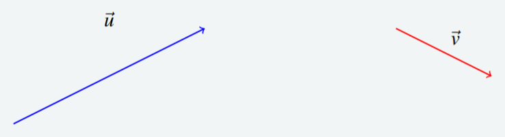
Considera los vectores\(\vec{u}\) y\(\vec{v}\) dibujados a continuación.

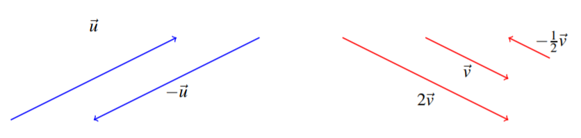
Dibujar\(-\vec{u}\),\(2\vec{v}\), y\(-\frac{1}{2}\vec{v}\).
Solución
Para encontrar\(-\vec{u}\), conservamos la longitud de\(\vec{u}\) y simplemente invertimos la dirección. Para\(2\vec{v}\), doblamos la longitud de\(\vec{v}\), conservando la dirección. Finalmente\(-\frac{1}{2}\vec{v}\) se encuentra tomando la mitad de la longitud de\(\vec{v}\) e invirtiendo la dirección. Estos vectores se muestran en el siguiente diagrama.

Ahora que hemos estudiado tanto la adición de vectores como la multiplicación escalar, podemos combinar las dos acciones. Recordar Definición 9.2.2 de combinaciones lineales de matrices de columna. Podemos aplicar esta definición a los vectores en\(\mathbb{R}^n\). Una combinación lineal de vectores en\(\mathbb{R}^n\) es una suma de vectores multiplicados por escalares.
En el siguiente ejemplo, examinamos el significado geométrico de este concepto.
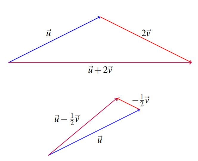
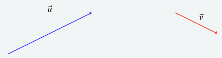
Considere la siguiente imagen de los vectores\(\vec{u}\) y\(\vec{v}\)

Esbozar una imagen de\(\vec{u}+2\vec{v},\vec{u}-\frac{1}{2}\vec{v}.\)
Solución
Los dos vectores se muestran a continuación.
