2.9: Cortes de rama y composición de funciones
- Page ID
- 109662
\( \newcommand{\vecs}[1]{\overset { \scriptstyle \rightharpoonup} {\mathbf{#1}} } \)
\( \newcommand{\vecd}[1]{\overset{-\!-\!\rightharpoonup}{\vphantom{a}\smash {#1}}} \)
\( \newcommand{\id}{\mathrm{id}}\) \( \newcommand{\Span}{\mathrm{span}}\)
( \newcommand{\kernel}{\mathrm{null}\,}\) \( \newcommand{\range}{\mathrm{range}\,}\)
\( \newcommand{\RealPart}{\mathrm{Re}}\) \( \newcommand{\ImaginaryPart}{\mathrm{Im}}\)
\( \newcommand{\Argument}{\mathrm{Arg}}\) \( \newcommand{\norm}[1]{\| #1 \|}\)
\( \newcommand{\inner}[2]{\langle #1, #2 \rangle}\)
\( \newcommand{\Span}{\mathrm{span}}\)
\( \newcommand{\id}{\mathrm{id}}\)
\( \newcommand{\Span}{\mathrm{span}}\)
\( \newcommand{\kernel}{\mathrm{null}\,}\)
\( \newcommand{\range}{\mathrm{range}\,}\)
\( \newcommand{\RealPart}{\mathrm{Re}}\)
\( \newcommand{\ImaginaryPart}{\mathrm{Im}}\)
\( \newcommand{\Argument}{\mathrm{Arg}}\)
\( \newcommand{\norm}[1]{\| #1 \|}\)
\( \newcommand{\inner}[2]{\langle #1, #2 \rangle}\)
\( \newcommand{\Span}{\mathrm{span}}\) \( \newcommand{\AA}{\unicode[.8,0]{x212B}}\)
\( \newcommand{\vectorA}[1]{\vec{#1}} % arrow\)
\( \newcommand{\vectorAt}[1]{\vec{\text{#1}}} % arrow\)
\( \newcommand{\vectorB}[1]{\overset { \scriptstyle \rightharpoonup} {\mathbf{#1}} } \)
\( \newcommand{\vectorC}[1]{\textbf{#1}} \)
\( \newcommand{\vectorD}[1]{\overrightarrow{#1}} \)
\( \newcommand{\vectorDt}[1]{\overrightarrow{\text{#1}}} \)
\( \newcommand{\vectE}[1]{\overset{-\!-\!\rightharpoonup}{\vphantom{a}\smash{\mathbf {#1}}}} \)
\( \newcommand{\vecs}[1]{\overset { \scriptstyle \rightharpoonup} {\mathbf{#1}} } \)
\( \newcommand{\vecd}[1]{\overset{-\!-\!\rightharpoonup}{\vphantom{a}\smash {#1}}} \)
\(\newcommand{\avec}{\mathbf a}\) \(\newcommand{\bvec}{\mathbf b}\) \(\newcommand{\cvec}{\mathbf c}\) \(\newcommand{\dvec}{\mathbf d}\) \(\newcommand{\dtil}{\widetilde{\mathbf d}}\) \(\newcommand{\evec}{\mathbf e}\) \(\newcommand{\fvec}{\mathbf f}\) \(\newcommand{\nvec}{\mathbf n}\) \(\newcommand{\pvec}{\mathbf p}\) \(\newcommand{\qvec}{\mathbf q}\) \(\newcommand{\svec}{\mathbf s}\) \(\newcommand{\tvec}{\mathbf t}\) \(\newcommand{\uvec}{\mathbf u}\) \(\newcommand{\vvec}{\mathbf v}\) \(\newcommand{\wvec}{\mathbf w}\) \(\newcommand{\xvec}{\mathbf x}\) \(\newcommand{\yvec}{\mathbf y}\) \(\newcommand{\zvec}{\mathbf z}\) \(\newcommand{\rvec}{\mathbf r}\) \(\newcommand{\mvec}{\mathbf m}\) \(\newcommand{\zerovec}{\mathbf 0}\) \(\newcommand{\onevec}{\mathbf 1}\) \(\newcommand{\real}{\mathbb R}\) \(\newcommand{\twovec}[2]{\left[\begin{array}{r}#1 \\ #2 \end{array}\right]}\) \(\newcommand{\ctwovec}[2]{\left[\begin{array}{c}#1 \\ #2 \end{array}\right]}\) \(\newcommand{\threevec}[3]{\left[\begin{array}{r}#1 \\ #2 \\ #3 \end{array}\right]}\) \(\newcommand{\cthreevec}[3]{\left[\begin{array}{c}#1 \\ #2 \\ #3 \end{array}\right]}\) \(\newcommand{\fourvec}[4]{\left[\begin{array}{r}#1 \\ #2 \\ #3 \\ #4 \end{array}\right]}\) \(\newcommand{\cfourvec}[4]{\left[\begin{array}{c}#1 \\ #2 \\ #3 \\ #4 \end{array}\right]}\) \(\newcommand{\fivevec}[5]{\left[\begin{array}{r}#1 \\ #2 \\ #3 \\ #4 \\ #5 \\ \end{array}\right]}\) \(\newcommand{\cfivevec}[5]{\left[\begin{array}{c}#1 \\ #2 \\ #3 \\ #4 \\ #5 \\ \end{array}\right]}\) \(\newcommand{\mattwo}[4]{\left[\begin{array}{rr}#1 \amp #2 \\ #3 \amp #4 \\ \end{array}\right]}\) \(\newcommand{\laspan}[1]{\text{Span}\{#1\}}\) \(\newcommand{\bcal}{\cal B}\) \(\newcommand{\ccal}{\cal C}\) \(\newcommand{\scal}{\cal S}\) \(\newcommand{\wcal}{\cal W}\) \(\newcommand{\ecal}{\cal E}\) \(\newcommand{\coords}[2]{\left\{#1\right\}_{#2}}\) \(\newcommand{\gray}[1]{\color{gray}{#1}}\) \(\newcommand{\lgray}[1]{\color{lightgray}{#1}}\) \(\newcommand{\rank}{\operatorname{rank}}\) \(\newcommand{\row}{\text{Row}}\) \(\newcommand{\col}{\text{Col}}\) \(\renewcommand{\row}{\text{Row}}\) \(\newcommand{\nul}{\text{Nul}}\) \(\newcommand{\var}{\text{Var}}\) \(\newcommand{\corr}{\text{corr}}\) \(\newcommand{\len}[1]{\left|#1\right|}\) \(\newcommand{\bbar}{\overline{\bvec}}\) \(\newcommand{\bhat}{\widehat{\bvec}}\) \(\newcommand{\bperp}{\bvec^\perp}\) \(\newcommand{\xhat}{\widehat{\xvec}}\) \(\newcommand{\vhat}{\widehat{\vvec}}\) \(\newcommand{\uhat}{\widehat{\uvec}}\) \(\newcommand{\what}{\widehat{\wvec}}\) \(\newcommand{\Sighat}{\widehat{\Sigma}}\) \(\newcommand{\lt}{<}\) \(\newcommand{\gt}{>}\) \(\newcommand{\amp}{&}\) \(\definecolor{fillinmathshade}{gray}{0.9}\)A menudo componemos funciones, i.e\(f(g(z))\). En general en este caso tenemos la regla de la cadena para calcular la derivada. Sin embargo, necesitamos especificar el dominio para\(z\) donde la función es analítica. Y cuando se trata de ramas y cortes de sucursales tenemos que cuidarnos.
Vamos\(f(z) = e^{z^2}\). Ya que\(e^z\) y\(z^2\) son ambas funciones enteras, así es\(f(z) = e^{z^2}\). La regla de la cadena nos da
\[f'(z) = e^{z^2} (2z).\]
Dejar\(f(z) = e^z\) y\(g(z) = 1/z\). \(f(z)\)es entero y\(g(z)\) es analítico en todas partes menos 0. Así\(f(g(z))\) es analítico excepto en 0 y
\(C\)- {\(2\pi n i\), donde\(n\) es cualquier entero}
La regla del cociente da\(h'(z) = -e^z/(e^z - 1)^2\). Un poco más formalmente:\(h(z) = f(g(z))\). dónde\(f(w) = 1/w\) y\(w = g(z) = e^z - 1\). Sabemos que\(g(z)\) es completo y\(f(w)\) es analítico en todas partes excepto\(w = 0\). Por lo tanto,\(f(g(z))\) es analítico en todas partes excepto en dónde\(g(z) = 0\).
Puede suceder que la derivada tenga un dominio mayor donde sea analítico que la función original. El ejemplo principal es\(f(z) = \log (z)\). Esto es analítico en\(C\) menos un corte de rama. Sin embargo
\[\dfrac{d}{dz} \log (z) = \dfrac{1}{z}\]
es analítico en\(C\) - {0}. Lo contrario no puede suceder.
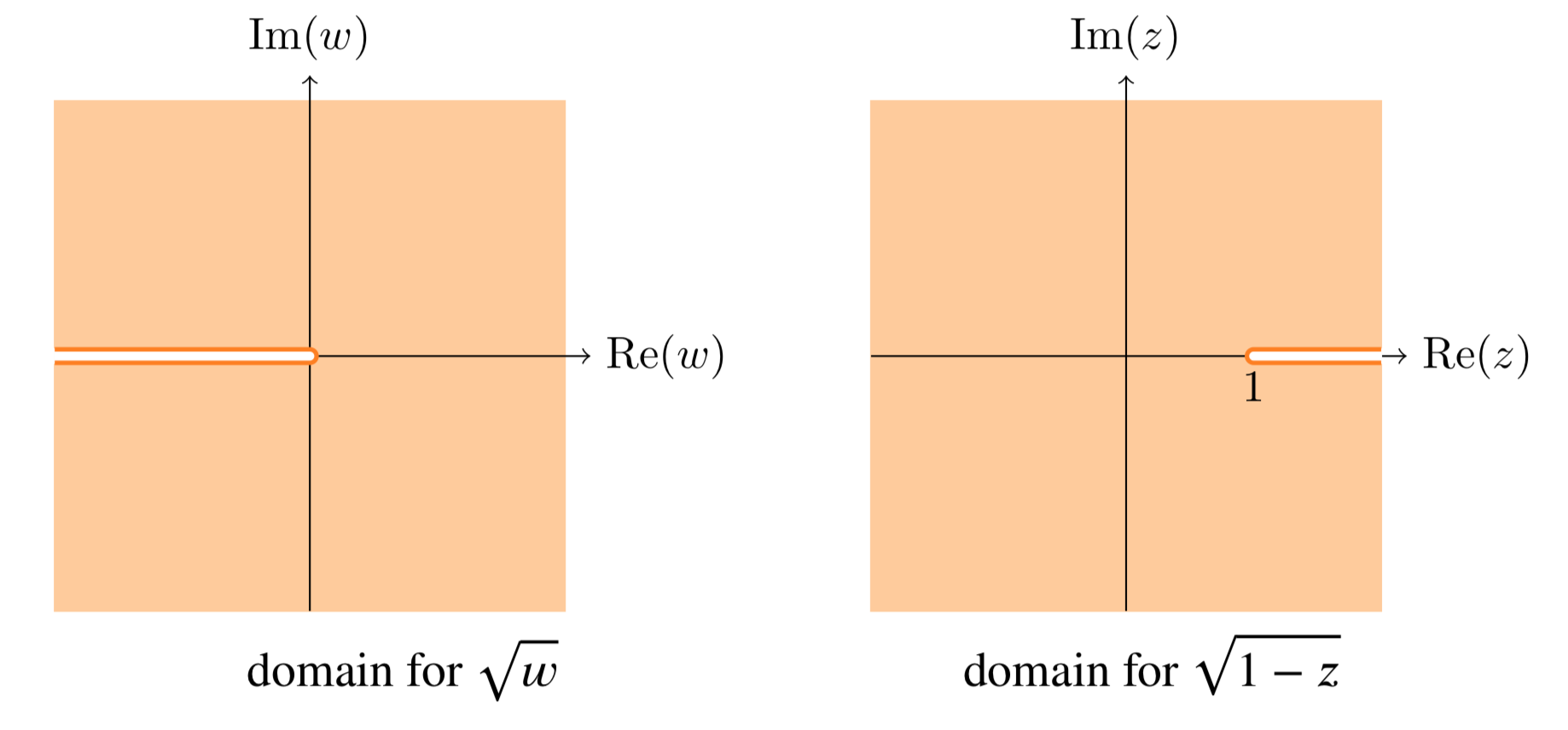
Definir una región donde\(\sqrt{1 - z}\) es analítica.
Solución
Elegir la rama principal del argumento, tenemos\(\sqrt{w}\) es analítico sobre
\(C - \{ x \le 0, y = 0\}\), (véase la figura a continuación.).
Así\(\sqrt{1 - z}\) es analítico excepto donde\(w = 1 - z\) está en el corte de rama, es decir, donde\(w = 1 - z\) es real y\(\le 0\). Es fácil ver que
\(w = 1 - z\)es real y\(\le 0\)\(\Leftrightarrow\)\(z\) es real y\(\ge 1\).
Así\(\sqrt{1 - z}\) es analítico en la región (ver figura abajo)
\[C - \{x \ge 1, y = 0\}\]
Una elección de rama diferente para\(\sqrt{w}\) conduciría a una región diferente donde\(\sqrt{1 - z}\) es analítica.
La siguiente figura muestra los dominios con cortes de rama para este ejemplo.
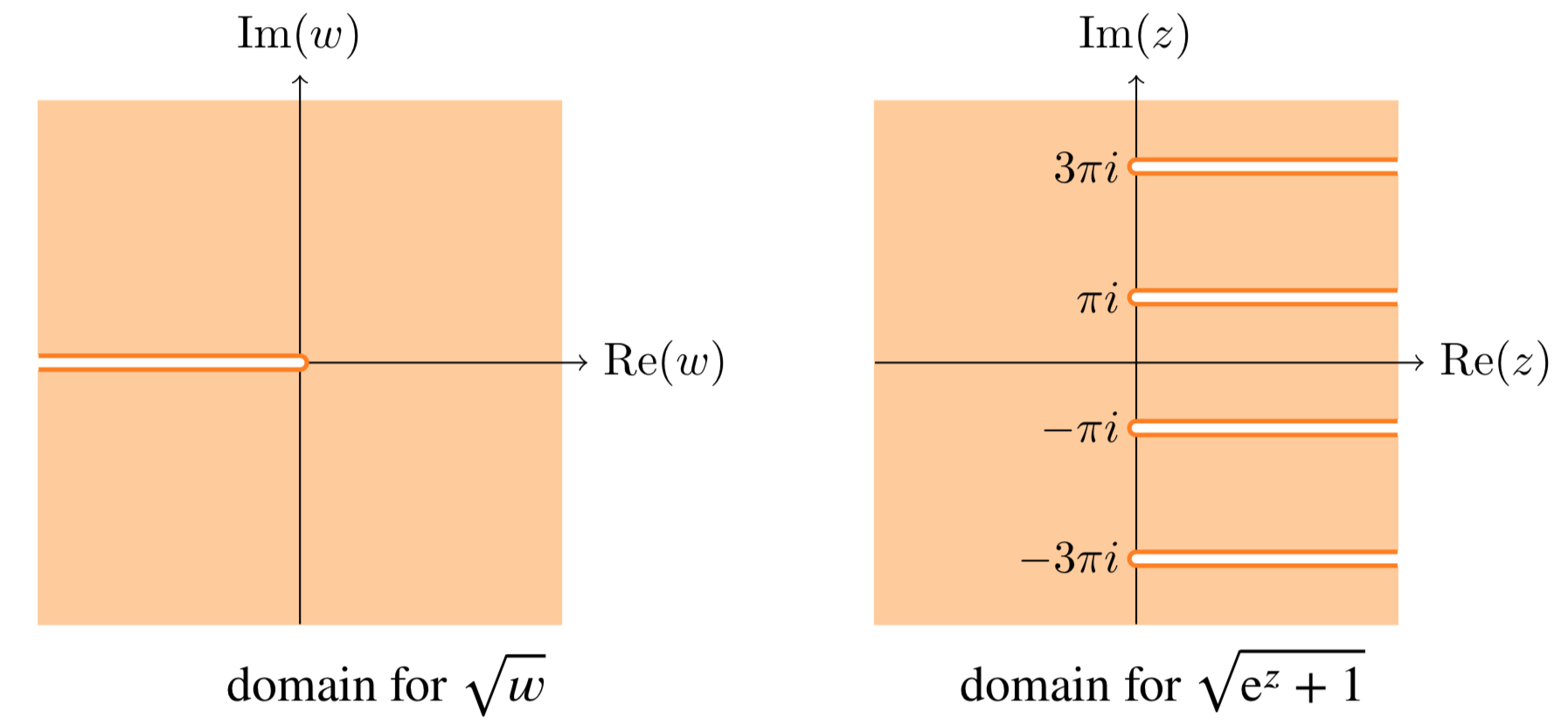
Definir una región donde\(f(z) = \sqrt{1 + e^z}\) es analítica.
Solución
Nuevamente, tomemos\(\sqrt{w}\) para ser analíticos en la región
\[C - \{x \le 0, y = 0\}\]
Entonces,\(f(z)\) es analítico excepto donde\(1 + e^z\) es real y\(\le 0\). Es decir, salvo donde\(e^z\) sea real y\(\le -1\). Ahora,\(e^z = e^x e^{iy}\) es real sólo cuando\(y\) es un múltiplo de\(\pi\). Es negativo solo cuando\(y\) es un mutltiple impar de\(\pi\). Tiene magnitud mayor a 1 sólo cuando\(x > 0\). Por lo tanto\(f(z)\) es analítico en la región
\[C - \{x \ge 0, y = \text{odd multiple of } \pi \}\]
La siguiente figura muestra los dominios con cortes de rama para este ejemplo.