2.2: PDE de Segundo Orden

Última actualización
Guardar como PDF

Page ID: 113859

\( \newcommand{\vecs}[1]{\overset { \scriptstyle \rightharpoonup} {\mathbf{#1}} } \) \( \newcommand{\vecd}[1]{\overset{-\!-\!\rightharpoonup}{\vphantom{a}\smash {#1}}} \)\(\newcommand{\id}{\mathrm{id}}\) \( \newcommand{\Span}{\mathrm{span}}\) \( \newcommand{\kernel}{\mathrm{null}\,}\) \( \newcommand{\range}{\mathrm{range}\,}\) \( \newcommand{\RealPart}{\mathrm{Re}}\) \( \newcommand{\ImaginaryPart}{\mathrm{Im}}\) \( \newcommand{\Argument}{\mathrm{Arg}}\) \( \newcommand{\norm}[1]{\| #1 \|}\) \( \newcommand{\inner}[2]{\langle #1, #2 \rangle}\) \( \newcommand{\Span}{\mathrm{span}}\) \(\newcommand{\id}{\mathrm{id}}\) \( \newcommand{\Span}{\mathrm{span}}\) \( \newcommand{\kernel}{\mathrm{null}\,}\) \( \newcommand{\range}{\mathrm{range}\,}\) \( \newcommand{\RealPart}{\mathrm{Re}}\) \( \newcommand{\ImaginaryPart}{\mathrm{Im}}\) \( \newcommand{\Argument}{\mathrm{Arg}}\) \( \newcommand{\norm}[1]{\| #1 \|}\) \( \newcommand{\inner}[2]{\langle #1, #2 \rangle}\) \( \newcommand{\Span}{\mathrm{span}}\)\(\newcommand{\AA}{\unicode[.8,0]{x212B}}\)

Los P.D.E. de segundo orden suelen dividirse en tres tipos. Demostremos esto para una PDE bidimensional general:

\[a\frac{\partial^2 u}{\partial x^2} +2c\frac{\partial^2 u}{\partial x \partial y} + b \frac{\partial^2 u}{\partial y^2} + d\frac{\partial u}{\partial x}+e\frac{\partial u}{\partial y}+f u+g=0 \nonumber \]

donde los coeficientes (es decir,\(a,\ldots,g\)) pueden ser constantes o funciones dadas de\(x,y\). Si\(g\) es 0 el sistema se llama homogéneo, de lo contrario se llama no homogéneo. Ahora se dice que la ecuación diferencial es

\[\left. \begin{array}{r} \text{elliptic}\\ \text{hyperbolic}\\ \text{parabolic} \end{array}\right\} \text{ if } \Delta(x,y) = ab-c^2 {\rm~is~} \left\{ \begin{array}{l} \text{positive}\\ \text{negative}\\ \text{zero} \end{array} \right. \nonumber \]

Razón detrás de los nombres

¿Por qué usamos estos nombres? La idea se explica con mayor facilidad para un caso con coeficientes constantes, y corresponde a una clasificación de la forma cuadrática asociada (reemplazar w.r.t. derivada\(x\) y\(y\) con\(\xi\) y\(\eta\))\[a\xi^2+b\eta^2+2c\xi\eta+f=0 \nonumber \]

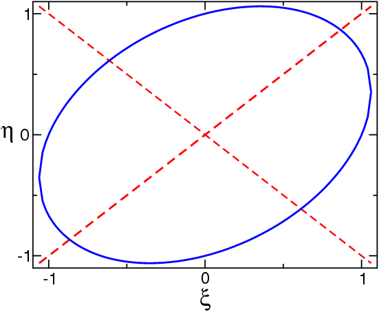
Descuidamos\(d\) y\(e\) ya que solo describen un desplazamiento del origen. Tal ecuación cuadrática puede describir cualquiera de las figuras geométricas discutidas anteriormente. Déjenme mostrar un ejemplo,\(a=3, b=3, c=1\) y\(f=−3\). Ya que\(ab−c^2=8\), esto debería describir una elipse. Podemos escribir

\[3\xi^2+3\eta^2+2\xi\eta=4 \left(\frac{\xi+\eta}{\sqrt{2}}\right)^2+2 \left(\frac{\xi-\eta}{\sqrt{2}}\right)^2=3 \label{4} \]

que es de hecho la ecuación de una elipse, con ejes girados, como puede verse en la Figura\(\PageIndex{1}\)

1 2.png — Figura\(\PageIndex{1}\): La elipse correspondiente a la Ecuación\ ref {4}.

También debemos darnos cuenta que la Ecuación\ ref {4} se puede escribir en la forma\[(\xi,\eta)\left (\array{3&1 \cr 1 &3} \right )\left (\array{\xi\cr\eta} \right) = 3 \nonumber \] vector-matriz-vector Ahora reconocemos que no\({\nabla}\) es más que el determinante de esta matriz, y es positivo si ambos valores propios son iguales, negativos si difieren en signo, y cero si uno de ellos es cero. (Nota: la elipse más simple corresponde a\(x^2+ y^2= 1\), una parábola a\(y= x^2\), y una hipérbola a\(x^2− y^2= 1\)).