Saltar al contenido principal
LibreTexts Español

10.8: Serie Fourier-Bessel

  • Page ID
    113677
  • \( \newcommand{\vecs}[1]{\overset { \scriptstyle \rightharpoonup} {\mathbf{#1}} } \)

    \( \newcommand{\vecd}[1]{\overset{-\!-\!\rightharpoonup}{\vphantom{a}\smash {#1}}} \)

    \( \newcommand{\id}{\mathrm{id}}\) \( \newcommand{\Span}{\mathrm{span}}\)

    ( \newcommand{\kernel}{\mathrm{null}\,}\) \( \newcommand{\range}{\mathrm{range}\,}\)

    \( \newcommand{\RealPart}{\mathrm{Re}}\) \( \newcommand{\ImaginaryPart}{\mathrm{Im}}\)

    \( \newcommand{\Argument}{\mathrm{Arg}}\) \( \newcommand{\norm}[1]{\| #1 \|}\)

    \( \newcommand{\inner}[2]{\langle #1, #2 \rangle}\)

    \( \newcommand{\Span}{\mathrm{span}}\)

    \( \newcommand{\id}{\mathrm{id}}\)

    \( \newcommand{\Span}{\mathrm{span}}\)

    \( \newcommand{\kernel}{\mathrm{null}\,}\)

    \( \newcommand{\range}{\mathrm{range}\,}\)

    \( \newcommand{\RealPart}{\mathrm{Re}}\)

    \( \newcommand{\ImaginaryPart}{\mathrm{Im}}\)

    \( \newcommand{\Argument}{\mathrm{Arg}}\)

    \( \newcommand{\norm}[1]{\| #1 \|}\)

    \( \newcommand{\inner}[2]{\langle #1, #2 \rangle}\)

    \( \newcommand{\Span}{\mathrm{span}}\) \( \newcommand{\AA}{\unicode[.8,0]{x212B}}\)

    \( \newcommand{\vectorA}[1]{\vec{#1}}      % arrow\)

    \( \newcommand{\vectorAt}[1]{\vec{\text{#1}}}      % arrow\)

    \( \newcommand{\vectorB}[1]{\overset { \scriptstyle \rightharpoonup} {\mathbf{#1}} } \)

    \( \newcommand{\vectorC}[1]{\textbf{#1}} \)

    \( \newcommand{\vectorD}[1]{\overrightarrow{#1}} \)

    \( \newcommand{\vectorDt}[1]{\overrightarrow{\text{#1}}} \)

    \( \newcommand{\vectE}[1]{\overset{-\!-\!\rightharpoonup}{\vphantom{a}\smash{\mathbf {#1}}}} \)

    \( \newcommand{\vecs}[1]{\overset { \scriptstyle \rightharpoonup} {\mathbf{#1}} } \)

    \( \newcommand{\vecd}[1]{\overset{-\!-\!\rightharpoonup}{\vphantom{a}\smash {#1}}} \)

    \(\newcommand{\avec}{\mathbf a}\) \(\newcommand{\bvec}{\mathbf b}\) \(\newcommand{\cvec}{\mathbf c}\) \(\newcommand{\dvec}{\mathbf d}\) \(\newcommand{\dtil}{\widetilde{\mathbf d}}\) \(\newcommand{\evec}{\mathbf e}\) \(\newcommand{\fvec}{\mathbf f}\) \(\newcommand{\nvec}{\mathbf n}\) \(\newcommand{\pvec}{\mathbf p}\) \(\newcommand{\qvec}{\mathbf q}\) \(\newcommand{\svec}{\mathbf s}\) \(\newcommand{\tvec}{\mathbf t}\) \(\newcommand{\uvec}{\mathbf u}\) \(\newcommand{\vvec}{\mathbf v}\) \(\newcommand{\wvec}{\mathbf w}\) \(\newcommand{\xvec}{\mathbf x}\) \(\newcommand{\yvec}{\mathbf y}\) \(\newcommand{\zvec}{\mathbf z}\) \(\newcommand{\rvec}{\mathbf r}\) \(\newcommand{\mvec}{\mathbf m}\) \(\newcommand{\zerovec}{\mathbf 0}\) \(\newcommand{\onevec}{\mathbf 1}\) \(\newcommand{\real}{\mathbb R}\) \(\newcommand{\twovec}[2]{\left[\begin{array}{r}#1 \\ #2 \end{array}\right]}\) \(\newcommand{\ctwovec}[2]{\left[\begin{array}{c}#1 \\ #2 \end{array}\right]}\) \(\newcommand{\threevec}[3]{\left[\begin{array}{r}#1 \\ #2 \\ #3 \end{array}\right]}\) \(\newcommand{\cthreevec}[3]{\left[\begin{array}{c}#1 \\ #2 \\ #3 \end{array}\right]}\) \(\newcommand{\fourvec}[4]{\left[\begin{array}{r}#1 \\ #2 \\ #3 \\ #4 \end{array}\right]}\) \(\newcommand{\cfourvec}[4]{\left[\begin{array}{c}#1 \\ #2 \\ #3 \\ #4 \end{array}\right]}\) \(\newcommand{\fivevec}[5]{\left[\begin{array}{r}#1 \\ #2 \\ #3 \\ #4 \\ #5 \\ \end{array}\right]}\) \(\newcommand{\cfivevec}[5]{\left[\begin{array}{c}#1 \\ #2 \\ #3 \\ #4 \\ #5 \\ \end{array}\right]}\) \(\newcommand{\mattwo}[4]{\left[\begin{array}{rr}#1 \amp #2 \\ #3 \amp #4 \\ \end{array}\right]}\) \(\newcommand{\laspan}[1]{\text{Span}\{#1\}}\) \(\newcommand{\bcal}{\cal B}\) \(\newcommand{\ccal}{\cal C}\) \(\newcommand{\scal}{\cal S}\) \(\newcommand{\wcal}{\cal W}\) \(\newcommand{\ecal}{\cal E}\) \(\newcommand{\coords}[2]{\left\{#1\right\}_{#2}}\) \(\newcommand{\gray}[1]{\color{gray}{#1}}\) \(\newcommand{\lgray}[1]{\color{lightgray}{#1}}\) \(\newcommand{\rank}{\operatorname{rank}}\) \(\newcommand{\row}{\text{Row}}\) \(\newcommand{\col}{\text{Col}}\) \(\renewcommand{\row}{\text{Row}}\) \(\newcommand{\nul}{\text{Nul}}\) \(\newcommand{\var}{\text{Var}}\) \(\newcommand{\corr}{\text{corr}}\) \(\newcommand{\len}[1]{\left|#1\right|}\) \(\newcommand{\bbar}{\overline{\bvec}}\) \(\newcommand{\bhat}{\widehat{\bvec}}\) \(\newcommand{\bperp}{\bvec^\perp}\) \(\newcommand{\xhat}{\widehat{\xvec}}\) \(\newcommand{\vhat}{\widehat{\vvec}}\) \(\newcommand{\uhat}{\widehat{\uvec}}\) \(\newcommand{\what}{\widehat{\wvec}}\) \(\newcommand{\Sighat}{\widehat{\Sigma}}\) \(\newcommand{\lt}{<}\) \(\newcommand{\gt}{>}\) \(\newcommand{\amp}{&}\) \(\definecolor{fillinmathshade}{gray}{0.9}\)

    Entonces, ¿cómo podemos determinar en general los coeficientes en la serie Fourier-Bessel?

    \[f(\rho) = \sum_{j=1}^\infty C_j J_\nu(\alpha_j \rho)? \nonumber \]

    Se encuentra fácilmente que la versión autoadjoint correspondiente de la ecuación de Bessel es (con\(R_j(\rho) = J_\nu(\alpha_j\rho)\))

    \[(\rho R_j')' + (\alpha_j^2\rho - \frac{\nu^2}{\rho}) R_j = 0. \nonumber \]

    Donde asumimos eso\(f\) y\(R\) satisfacemos la condición límite

    \[\begin{aligned} b_1 f(c) + b_2 f'(c) &= 0 \nonumber\\ b_1 R_j(c) + b_2 R_j'(c) & = & 0 \end{aligned} \nonumber \]

    De la teoría de Sturm-Liouville sí lo sabemos\[\int_0^c \rho J_\nu(\alpha_i \rho) J_\nu(\alpha_j \rho) = 0 \;\;{\rm if\ }i \neq j, \nonumber \] pero también necesitaremos los valores cuando\(i=j\)!

    Usemos la forma autoadjoint de la ecuación, y multipliquemos con\(2 \rho R'\), e integremos\(\rho\) de\(0\) a\(c\),

    \[\int_0^c \left[(\rho R_j')' + (\alpha_j^2\rho - \frac{\nu^2}{\rho}) R_j \right]2 \rho R_j' d\rho = 0. \nonumber \]

    Esto se puede llevar a la forma (integrar el primer término por partes, llevar los otros dos términos al lado derecho)

    \[\begin{aligned} \int_0^c \frac{d}{d\rho}\left(\rho R_j'\right)^2 d\rho &= 2 \nu^2 \int_0^c R_j R_j' d\rho -2\alpha_j^2 \int_0^c \rho^2 R_j R_j' d\rho\\ \left.\left(\rho R_j'\right)^2\right|^c_0 &= \left.\nu^2 R_j^2\right|^c_0 - 2\alpha_j^2 \int_0^c \rho^2 R_j R_j' d\rho.\end{aligned} \nonumber \]

    La última integral ahora se puede hacer por partes:\[\begin{aligned} 2 \int_0^c\rho^2 R_j R_j' d\rho &= -2 \int_0^c\rho R_j^2 d\rho +\left. \rho R_j^2 \right|^c_0.\end{aligned} \nonumber \]

    Así que finalmente concluimos que

    \[2 \alpha_j^2 \int_0^c\rho R_j^2 d\rho = \left[\left(\alpha_j^2\rho^2 - \nu^2 \right) R_j^2+\left(\rho R_j'\right)^2 \right|^c_0. \nonumber \]

    Para que la vida no sea demasiado complicada solo veremos las condiciones limítrofes donde\(f(c)=R(c)=0\). ¡Los otros casos (mixtos o puramente\(f'(c)=0\)) van muy parecidos! Utilizando el hecho de que\(R_j(r) = J_\nu(\alpha_j \rho)\), encontramos\[R'_j=\alpha_j J'_\nu(\alpha_j \rho). \nonumber \] Concluimos que

    \[\begin{aligned} 2 \alpha_j^2 \int_0^c\rho^2 R_j^2 d\rho &= \left[ \left(\rho \alpha_j J'_\nu(\alpha_j\rho)\right)^2 \right|^c_0 \nonumber\\ &= {c^2}\alpha_j^2 \left(J'_\nu(\alpha_j c)\right)^2 \nonumber\\ &= {c^2}\alpha_j^2 \left(\frac{\nu}{\alpha_j c} J_\nu(\alpha_j c) -J_{\nu+1}(\alpha_j c)\right)^2 \nonumber\\ &= {c^2}\alpha_j^2 \left( J_{\nu+1}(\alpha_j c)\right)^2 ,\end{aligned} \nonumber \]

    Así finalmente tenemos el resultado\[\int_0^c\rho^2 R_j^2 d\rho=\frac{c^2}{2} J^2_{\nu+1}(\alpha_j c). \nonumber \]

    Ejemplo\(\PageIndex{1}\):

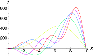
    Considera la función

    \[f(x) = \left\{\begin{array}{ll} x^3 &\;\;0<x<10\\ 0&\;\;x>10 \end{array}\right. \nonumber \]

    Expanda esta función en una serie de Fourier-Bessel usando\(J_3\).

    Solución

    De nuestras definiciones encontramos que

    \[f(x) = \sum_{j=1}^\infty A_j J_3(\alpha_j x), \nonumber \]

    con

    \[\begin{aligned} A_j &= \frac{2}{100 J_4(10\alpha_j)^2} \int_0^{10} x^3 J_3(\alpha_j x) dx\nonumber\\ &=\frac{2}{100 J_4(10\alpha_j)^2} \frac{1}{\alpha^5_j} \int_0^{10\alpha_j} s^4 J_3(s) ds\nonumber\\ &=\frac{2}{100 J_4(10\alpha_j)^2} \frac{1}{\alpha^5_j} (10 \alpha_j)^4 J_4(10\alpha_j ) ds\nonumber\\ &= \frac{200}{\alpha_j J_4(10 \alpha_j)}.\end{aligned} \nonumber \]

    Utilizando\(\alpha_j=\ldots\), encontramos que los primeros cinco valores de\(A_j\) son\(1050.95,-821.503,703.991,-627.577,572.301\). Las primeras cinco sumas parciales se representan gráficamente en la Fig. \(\PageIndex{1}\).

    Besselx3.png
    Figura\(\PageIndex{1}\): Una gráfica de las primeras cinco sumas parciales para\(x^3\) expresado en\(J_3\).

    This page titled 10.8: Serie Fourier-Bessel is shared under a CC BY-NC-SA 2.0 license and was authored, remixed, and/or curated by Niels Walet via source content that was edited to the style and standards of the LibreTexts platform.