
6.2: Resolver ecuaciones de valores absolutos
- Page ID
- 112577
Para resolver ecuaciones de valor absoluto, primero considere las siguientes dos propiedades de valor absoluto:
Propiedad 1: Para\(b > 0\),\(|a| = b\) si y solo si\(a = b\) o\(a = −b\)
Propiedad 2: Para cualquier número real\(a\) y\(b\),\(|a| = |b|\) si y solo si\(a = b\) o\(a = −b\)
- Antes de aplicar la Propiedad 1, aísle la expresión de valor absoluto a cada lado de la ecuación.
- Verifique las soluciones sustituyéndolas de nuevo en la ecuación original.
- Las soluciones se presentan como un conjunto de soluciones de la forma\(\{p, q\}\), donde\(p\) y\(q\) son los números reales.
- El conjunto de soluciones de una ecuación de valor absoluto se grafica como puntos en una recta numérica.
Resuelve cada ecuación y grafica el conjunto de soluciones.
- \(|x| = 7\)
- \(|5x – 3| = 2\)
- \(|20 – x| = −80\)
Solución
- Para resolver\(|x| = 7\), aplicar Inmueble 1 con\(a = x\) y\(b = 7\).
Por lo tanto, las soluciones son,\(x = −7\) y\(x = 7\), y el conjunto de soluciones es\(\{-7,7\}\). El gráfico del conjunto de soluciones es como se muestra en la siguiente figura.

- El método de resolución de ecuaciones utilizado en la parte a se puede extender a la ecuación dada en esta parte con\(a = 5x – 3\) y\(b = 2\).
Así, la ecuación del valor absoluto\(|5x – 3| = 2\) es equivalente a:
\(\begin{array} &&5x − 3 = 2 &\text{ or } &5x − 3 = −2 &\text{Property 1} \\ &5x = 5 &\text{ or } &5x = 1 &\text{Add \(3\)a ambos lados de las ecuaciones}\\ &x = 1 &\ text {o} &x =\ dfrac {1} {5} &\ text {Dividir por\(5\) ambos lados de las ecuaciones}\ end {array}\)
Ahora, verifique si\(x = 1\) y\(x = \dfrac{1}{5}\) son soluciones a la ecuación de valor absoluto dada.
\(\begin{array} &&\text{For } x = 1 &\text{For } x = \dfrac{1}{5} &\\ &|5x − 3| = 2 &|5x − 3| = 2 &\text{Given} \\ &|5(1) − 3| \stackrel{?}{=} 2 &|5 \left( \dfrac{1}{5} \right) − 3| \stackrel{?}{=} 2 &\text{Substitute the \(x\)-valores}\\ &|5 − 3|\ stackrel {?} {=} 2 &|1 − 3|\ stackrel {?} {=} 2 &\ text {Simplificar}\\ &|2|\ stackrel {?} {=} 2 &|− 2|\ stackrel {?} {=} 2 &\ text {Aplicar la definición del valor absoluto}\\ &2 = 2\;\ checkmark &2 = 2\;\ checkmark\ end {array}\)
Dado que las ecuaciones anteriores son verdaderas, entonces,\(x = 1\) y\(x = \dfrac{1}{5}\) son soluciones a la ecuación de valor absoluto dada. El conjunto de soluciones es\(\left\{\dfrac{1}{5} , 1\right\}\). El gráfico del conjunto de soluciones es como se muestra en la siguiente figura.

- Dado que un valor absoluto nunca puede ser negativo, no hay números reales\(x\) que hagan\(|20 – x| = −80\) realidad. La ecuación no tiene solución y el conjunto de soluciones es\(∅\).
Resuelve y grafica el conjunto de soluciones.
- \(\left| \dfrac{4}{3} x + 3 \right| + 8 = 18\)
- \(4 \left| \dfrac{1}{3}x − 6 \right| − 5 = −5\)
- \(|4x – 3| = |x + 6|\)
Solución
- Observe que la expresión de valor absoluto no está aislada, lo que significa que no se pueden aplicar las propiedades. Primero, aísle\(\left| \dfrac{4}{3}x + 3 \right|\) en el lado izquierdo de la ecuación, luego, aplique la Propiedad 1.
\(\begin{array} &&\left| \dfrac{4}{3} x + 3 \right| + 8 = 18 &\text{Given equation} \\ & \left| \dfrac{4}{3} + 3 \right| = 10 &\text{Subtract \(8\)desde ambos lados de la ecuación}\ end {array}\)
Con el valor absoluto ahora aislado, resuelva\(\left| \dfrac{4}{3} + 3 \right| = 10\) usando la Propiedad 1, con\(a = \dfrac{4}{3} x + 3\) y de la\(b = 10\) siguiente manera,
\(\begin{array} && &\left| \dfrac{4}{3} + 3 \right| = 10 & & \\ &\dfrac{4}{3} + 3 = 10 &\text{ or } & \dfrac{4}{3} + 3 = -10 &\text{Property 1} \\ &\dfrac{4}{3} x = 7 &\text{ or } &\dfrac{4}{3}x = −13 &\text{Subtract \(3\)desde ambos lados}\\ &x =\ dfrac {21} {4} &\ text {o} &x = −\ dfrac {39} {4} &\ text {Multiplicar ambos lados por\(\dfrac{3}{4}\)}\ end {array}\)
Verifique las soluciones\(x = −\dfrac{39}{4}\) y\(x = \dfrac{21}{4}\) sustituyéndolas en la ecuación de valor absoluto original. El conjunto de soluciones es\(\left\{ −\dfrac{39}{4}, \dfrac{21}{4} \right\}\) y la gráfica del conjunto de soluciones es como se muestra en la siguiente figura.

- Similar a la parte a, aísle la expresión de valor absoluto. Entonces, primero aísle\(\left| \dfrac{1}{3} x − 6 \right|\) en el lado izquierdo de la ecuación y aplique la Propiedad 1.
\(\begin{array} &&4 \left| \dfrac{1}{3}x − 6 \right| − 5 = −5 &\text{Given equation} \\ &4 \left| \dfrac{1}{3}x − 6 \right| = 0 &\text{Add \(5\)a ambos lados de la ecuación}\\ &\ izquierda|\ dfrac {1} {3} x − 6\ derecha| = 0 &\ text {Dividir por\(4\) ambos lados de la ecuación}\ end {array}\)
El valor absoluto está aislado. Dado que\(0\) es el único número cuyo valor absoluto es\(0\), la expresión\(\dfrac{1}{3}x − 6\) debe ser igual a\(0\). Entonces,
\(\begin{array} &&\dfrac{1}{3}x − 6 = 0 & \\ &\dfrac{1}{3}x − 6 &\text{Add \(6\)a ambos lados de la ecuación}\\ &x = 18 &\ text {Multiplicar ambos lados por\(3\)}\ end {array}\)
La solución es\(18\) y el conjunto de soluciones es\(\{18\}\). Verificar que satisfaga la ecuación original. El gráfico del conjunto de soluciones es como se muestra en la siguiente figura.

- \(|4x − 7| = |x + 14|\)Observe que para resolver\(|4x − 7| = |x + 14|\), use Inmueble 2 con\(a = 4x − 7\) y\(b = x + 14\).
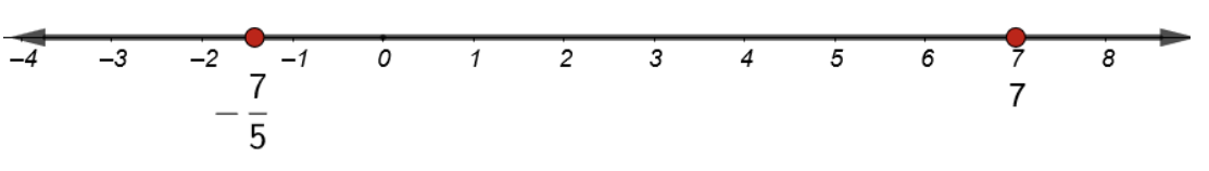
\(\begin{array} && &|4x − 7| = |x + 14| & &\text{Given} \\ &4x−7 = x+14 &\text{ or } &4x − 7 = −(x + 14) &\text{Property 2} \\ &4x−7 = x+14 &\text{ or } &4x − 7 = −x − 14 &\text{Distribute \(−1\)para simplificar la ecuación correcta}\\ &4x = x + 21 &\ text {o} &4x = −x − 7 &\ text {Añadir\(7\) a ambos lados de cada igualdad}\\ &3x = 21 &\ text {o} &5x = −7 &\ text {Simplificar}\\ &x = 7 &\ text {o} &x = −\ dfrac {7} {5} &\ text {Divide cada ecuación por el\(x\) -coeficiente}\ end {array}\)
Verifique las soluciones\(x = −\dfrac{7}{5}\) y\(x = 7\) sustituyéndolas en la ecuación de valor absoluto original. El conjunto de soluciones es\(\left\{ −\dfrac{7}{5}, 7\right\}\). El gráfico de la solución es como se muestra en la siguiente figura.
Resuelve cada ecuación, comprueba la solución y grafica el conjunto de soluciones.
- \(|x| = 19\)
- \(|x − 4| = 10\)
- \(|2x − 5| = 12\)
- \(\left|\dfrac{x}{11} \right| = 2.5\)
- \(|x − 3.8| = −2.7\)
- \(|3x − 4.5| = 9.3\)
- \(\dfrac{8}{3} |x − 6| = 14\)
- \(|x + 15| − 19 = 7\)
- \(|11x + 3| + 28 = 16\)
- \( \left| \dfrac{8}{7} x + 9 \right| − 2 = 8\)
- \( −3|2x − 7| + 13 = 13\)
- \( 8 − 5|10x + 6| = 5\)
- \( |5x − 14| = |3x − 9|\)
- \( |15x| = |x − 21|\)
- \( |4x − 7| = |5(2x + 3)|\)
- \( \dfrac{7}{8} = \dfrac{3x}{2} + \dfrac{2x}{5}\)