11.9: Flujos alrededor de los cilindros
- Page ID
- 109901
\( \newcommand{\vecs}[1]{\overset { \scriptstyle \rightharpoonup} {\mathbf{#1}} } \)
\( \newcommand{\vecd}[1]{\overset{-\!-\!\rightharpoonup}{\vphantom{a}\smash {#1}}} \)
\( \newcommand{\id}{\mathrm{id}}\) \( \newcommand{\Span}{\mathrm{span}}\)
( \newcommand{\kernel}{\mathrm{null}\,}\) \( \newcommand{\range}{\mathrm{range}\,}\)
\( \newcommand{\RealPart}{\mathrm{Re}}\) \( \newcommand{\ImaginaryPart}{\mathrm{Im}}\)
\( \newcommand{\Argument}{\mathrm{Arg}}\) \( \newcommand{\norm}[1]{\| #1 \|}\)
\( \newcommand{\inner}[2]{\langle #1, #2 \rangle}\)
\( \newcommand{\Span}{\mathrm{span}}\)
\( \newcommand{\id}{\mathrm{id}}\)
\( \newcommand{\Span}{\mathrm{span}}\)
\( \newcommand{\kernel}{\mathrm{null}\,}\)
\( \newcommand{\range}{\mathrm{range}\,}\)
\( \newcommand{\RealPart}{\mathrm{Re}}\)
\( \newcommand{\ImaginaryPart}{\mathrm{Im}}\)
\( \newcommand{\Argument}{\mathrm{Arg}}\)
\( \newcommand{\norm}[1]{\| #1 \|}\)
\( \newcommand{\inner}[2]{\langle #1, #2 \rangle}\)
\( \newcommand{\Span}{\mathrm{span}}\) \( \newcommand{\AA}{\unicode[.8,0]{x212B}}\)
\( \newcommand{\vectorA}[1]{\vec{#1}} % arrow\)
\( \newcommand{\vectorAt}[1]{\vec{\text{#1}}} % arrow\)
\( \newcommand{\vectorB}[1]{\overset { \scriptstyle \rightharpoonup} {\mathbf{#1}} } \)
\( \newcommand{\vectorC}[1]{\textbf{#1}} \)
\( \newcommand{\vectorD}[1]{\overrightarrow{#1}} \)
\( \newcommand{\vectorDt}[1]{\overrightarrow{\text{#1}}} \)
\( \newcommand{\vectE}[1]{\overset{-\!-\!\rightharpoonup}{\vphantom{a}\smash{\mathbf {#1}}}} \)
\( \newcommand{\vecs}[1]{\overset { \scriptstyle \rightharpoonup} {\mathbf{#1}} } \)
\( \newcommand{\vecd}[1]{\overset{-\!-\!\rightharpoonup}{\vphantom{a}\smash {#1}}} \)
\(\newcommand{\avec}{\mathbf a}\) \(\newcommand{\bvec}{\mathbf b}\) \(\newcommand{\cvec}{\mathbf c}\) \(\newcommand{\dvec}{\mathbf d}\) \(\newcommand{\dtil}{\widetilde{\mathbf d}}\) \(\newcommand{\evec}{\mathbf e}\) \(\newcommand{\fvec}{\mathbf f}\) \(\newcommand{\nvec}{\mathbf n}\) \(\newcommand{\pvec}{\mathbf p}\) \(\newcommand{\qvec}{\mathbf q}\) \(\newcommand{\svec}{\mathbf s}\) \(\newcommand{\tvec}{\mathbf t}\) \(\newcommand{\uvec}{\mathbf u}\) \(\newcommand{\vvec}{\mathbf v}\) \(\newcommand{\wvec}{\mathbf w}\) \(\newcommand{\xvec}{\mathbf x}\) \(\newcommand{\yvec}{\mathbf y}\) \(\newcommand{\zvec}{\mathbf z}\) \(\newcommand{\rvec}{\mathbf r}\) \(\newcommand{\mvec}{\mathbf m}\) \(\newcommand{\zerovec}{\mathbf 0}\) \(\newcommand{\onevec}{\mathbf 1}\) \(\newcommand{\real}{\mathbb R}\) \(\newcommand{\twovec}[2]{\left[\begin{array}{r}#1 \\ #2 \end{array}\right]}\) \(\newcommand{\ctwovec}[2]{\left[\begin{array}{c}#1 \\ #2 \end{array}\right]}\) \(\newcommand{\threevec}[3]{\left[\begin{array}{r}#1 \\ #2 \\ #3 \end{array}\right]}\) \(\newcommand{\cthreevec}[3]{\left[\begin{array}{c}#1 \\ #2 \\ #3 \end{array}\right]}\) \(\newcommand{\fourvec}[4]{\left[\begin{array}{r}#1 \\ #2 \\ #3 \\ #4 \end{array}\right]}\) \(\newcommand{\cfourvec}[4]{\left[\begin{array}{c}#1 \\ #2 \\ #3 \\ #4 \end{array}\right]}\) \(\newcommand{\fivevec}[5]{\left[\begin{array}{r}#1 \\ #2 \\ #3 \\ #4 \\ #5 \\ \end{array}\right]}\) \(\newcommand{\cfivevec}[5]{\left[\begin{array}{c}#1 \\ #2 \\ #3 \\ #4 \\ #5 \\ \end{array}\right]}\) \(\newcommand{\mattwo}[4]{\left[\begin{array}{rr}#1 \amp #2 \\ #3 \amp #4 \\ \end{array}\right]}\) \(\newcommand{\laspan}[1]{\text{Span}\{#1\}}\) \(\newcommand{\bcal}{\cal B}\) \(\newcommand{\ccal}{\cal C}\) \(\newcommand{\scal}{\cal S}\) \(\newcommand{\wcal}{\cal W}\) \(\newcommand{\ecal}{\cal E}\) \(\newcommand{\coords}[2]{\left\{#1\right\}_{#2}}\) \(\newcommand{\gray}[1]{\color{gray}{#1}}\) \(\newcommand{\lgray}[1]{\color{lightgray}{#1}}\) \(\newcommand{\rank}{\operatorname{rank}}\) \(\newcommand{\row}{\text{Row}}\) \(\newcommand{\col}{\text{Col}}\) \(\renewcommand{\row}{\text{Row}}\) \(\newcommand{\nul}{\text{Nul}}\) \(\newcommand{\var}{\text{Var}}\) \(\newcommand{\corr}{\text{corr}}\) \(\newcommand{\len}[1]{\left|#1\right|}\) \(\newcommand{\bbar}{\overline{\bvec}}\) \(\newcommand{\bhat}{\widehat{\bvec}}\) \(\newcommand{\bperp}{\bvec^\perp}\) \(\newcommand{\xhat}{\widehat{\xvec}}\) \(\newcommand{\vhat}{\widehat{\vvec}}\) \(\newcommand{\uhat}{\widehat{\uvec}}\) \(\newcommand{\what}{\widehat{\wvec}}\) \(\newcommand{\Sighat}{\widehat{\Sigma}}\) \(\newcommand{\lt}{<}\) \(\newcommand{\gt}{>}\) \(\newcommand{\amp}{&}\) \(\definecolor{fillinmathshade}{gray}{0.9}\)Teorema del círculo de Milne-Thomson
El teorema de Milne-Thomson nos permite insertar un círculo en un flujo bidimensional y ver cómo se ajusta el flujo. Primero declararemos y probaremos el teorema.
Si\(f(z)\) es un potencial complejo con todas sus singularidades afuera\(|z| = R\) entonces
\[\Phi (z) = f(z) + \overline{f(\dfrac{R^2}{\overline{z}})}\]
es un potencial complejo con racionalidad\(|z| = R\) y las mismas singularidades que\(f\) en la región\(|z| > R\).
- Prueba
-
Primera nota que\(R^2/\overline{z}\) es el reflejo de\(z\) en el círculo\(|z| = R\).
A continuación tenemos que ver que\(\overline{f(R^2/\overline{z})}\) es analítico para\(|z| > R\). Por supuesto\(f(z)\) es analítico para\(|z| < R\), por lo que se puede expresar como una serie de Taylor
\[f(z) = a_0 + a_1 z + a_2 z^2 + \ ...\]
Por lo tanto,
\[\overline{f(\dfrac{R^2}{\overline{z}})} = \overline{a_0} + \overline{a_1} \dfrac{R^2}{z} + \overline{a_2} (\dfrac{R^2}{z})^2 + \ ...\]
Todas las singularidades de\(f\) están afuera\(|z| = R\), por lo que la serie Taylor en la Ecuación 11.10.2 converge para\(|z| \le R\). Esto significa que la serie Laurent en la Ecuación 11.10.3 converge para\(|z| \ge R\). Es decir,\(\overline{f(R^2/\overline{z})}\) es analítico\(|z| \ge R\), es decir, no introduce singulares al\(\Phi (z)\) exterior\(|z| = R\).
Lo último que hay que mostrar es que\(|z| = R\) es una racionalización para\(\Phi (z)\). Esto sigue porque para\(z = Re^{i \theta}\)
\[\Phi (Re^{i \theta}) = f(Re^{i \theta} + \overline{f(Re^{i \theta})}\]
es real. Por lo tanto
\[\psi (Re^{i \theta} = \text{Im} (\Phi (Re^{i \theta}) = 0.\]
Ejemplos
\(f(z)\)Piense en representar el flujo, posiblemente con fuentes o vórtices afuera\(|z| = R\). Entonces\(\Phi (z)\) representa el nuevo flujo cuando se coloca un obstáculo circular en el flujo. Aquí hay algunos ejemplos.
Sabemos por el Tema 6 que\(f(z) = z\) es el complejo potencial de flujo uniforme hacia la derecha. Entonces,
\[\Phi (z) = z + R^2/z\]
es el potencial de flujo uniforme alrededor de un círculo de radio\(R\) centrado en el origen.
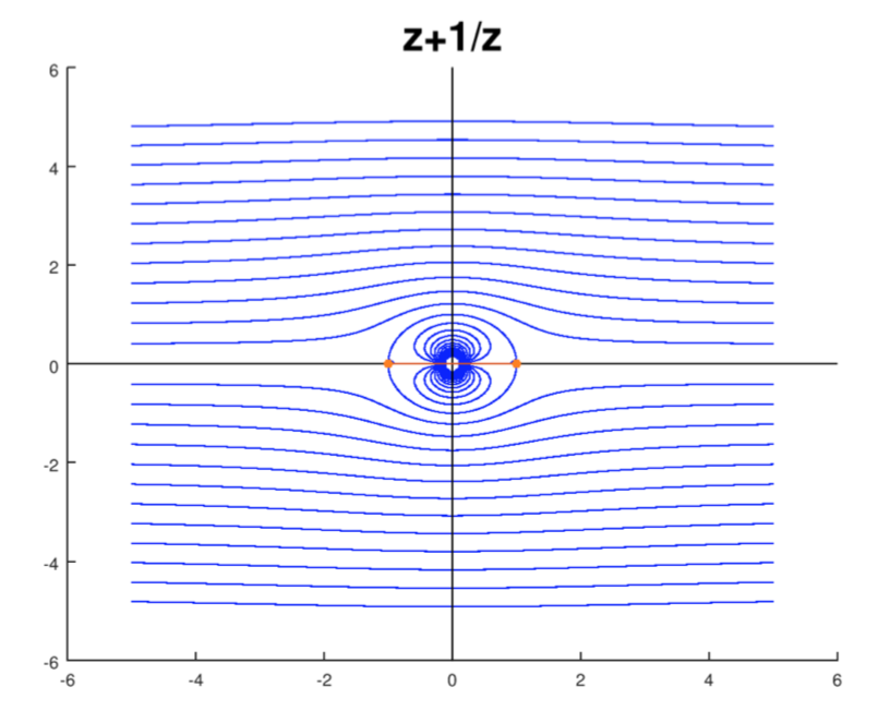
Flujo uniforme alrededor de un círculo
Sólo porque se ven bien, la figura incluye líneas de racionalización dentro del círculo. Estos no interactúan con el flujo fuera del círculo.
Tenga en cuenta que a medida que\(z\) obtiene un flujo grande se ve uniforme. Podemos ver esto analíticamente porque
\[\Phi '(z) = 1 - R^2/z^2\]
va a 1 como\(z\) se hace grande. (Recordemos que el campo de velocidad es (\(\phi _x, \phi _y\)), donde\(\Phi = \phi + i \psi \ ...\))
Aquí la fuente está en\(z = -2\) (fuera del círculo unitario) con potencial complejo
\[f(z) = \log (z + 2).\]
Con el corte de rama apropiado las singularidades de también\(f\) están afuera\(|z| = 1\). Así podemos aplicar Milne-Thomson y obtener
\[\Phi (z) = \log (z + 2) + \overline{\log (\dfrac{1}{\overline{z}} + 2)}\]
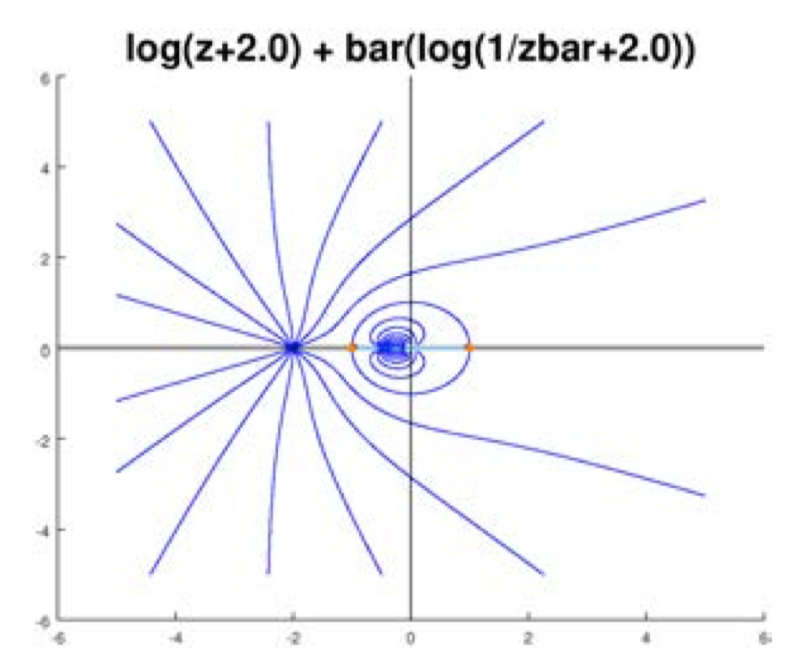
Flujo fuente alrededor de un círculo
Sabemos que lejos del origen el flujo debe verse igual que un flujo con solo una fuente\(z = -2\).
Veamos esto analíticamente. Primero señalamos un dato útil:
Si\(g(z)\) es analítico entonces así es\(h(z) = \overline{g(\overline{z})}\) y\(h'(z) = \overline{g'(\overline{z})}\).
- Prueba
-
Utilice la serie Taylor\(g\) para obtener la serie Taylor para\(h\) y luego compare\(h'(z)\) y\(\overline{g'(\overline{z})}\).
Usando esto tenemos
\[\Phi ' (z) = \dfrac{1}{z + 2} - \dfrac{1}{z(1 + 2z)}\]
Para grandes\(z\) el segundo término decae mucho más rápido que el primero, por lo que
\[\Phi ' (z) \approx \dfrac{1}{z + 2}.\]
Es decir, lejos de\(z = 0\), el campo de velocidad se parece al campo de velocidad para\(f(z)\), es decir, el campo de velocidad de una fuente en\(z = -2\).
Si usamos
\[g(z) = z^2\]
podemos transformar un flujo desde el semiplano superior al primer cuadrante
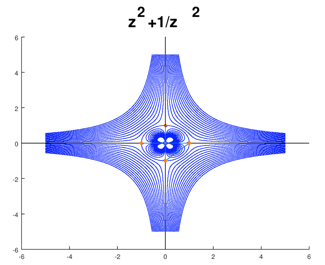
Flujo de origen alrededor de un cuarto de esquina circular