4.5: BM 13901 #12
- Page ID
- 109592
\( \newcommand{\vecs}[1]{\overset { \scriptstyle \rightharpoonup} {\mathbf{#1}} } \)
\( \newcommand{\vecd}[1]{\overset{-\!-\!\rightharpoonup}{\vphantom{a}\smash {#1}}} \)
\( \newcommand{\id}{\mathrm{id}}\) \( \newcommand{\Span}{\mathrm{span}}\)
( \newcommand{\kernel}{\mathrm{null}\,}\) \( \newcommand{\range}{\mathrm{range}\,}\)
\( \newcommand{\RealPart}{\mathrm{Re}}\) \( \newcommand{\ImaginaryPart}{\mathrm{Im}}\)
\( \newcommand{\Argument}{\mathrm{Arg}}\) \( \newcommand{\norm}[1]{\| #1 \|}\)
\( \newcommand{\inner}[2]{\langle #1, #2 \rangle}\)
\( \newcommand{\Span}{\mathrm{span}}\)
\( \newcommand{\id}{\mathrm{id}}\)
\( \newcommand{\Span}{\mathrm{span}}\)
\( \newcommand{\kernel}{\mathrm{null}\,}\)
\( \newcommand{\range}{\mathrm{range}\,}\)
\( \newcommand{\RealPart}{\mathrm{Re}}\)
\( \newcommand{\ImaginaryPart}{\mathrm{Im}}\)
\( \newcommand{\Argument}{\mathrm{Arg}}\)
\( \newcommand{\norm}[1]{\| #1 \|}\)
\( \newcommand{\inner}[2]{\langle #1, #2 \rangle}\)
\( \newcommand{\Span}{\mathrm{span}}\) \( \newcommand{\AA}{\unicode[.8,0]{x212B}}\)
\( \newcommand{\vectorA}[1]{\vec{#1}} % arrow\)
\( \newcommand{\vectorAt}[1]{\vec{\text{#1}}} % arrow\)
\( \newcommand{\vectorB}[1]{\overset { \scriptstyle \rightharpoonup} {\mathbf{#1}} } \)
\( \newcommand{\vectorC}[1]{\textbf{#1}} \)
\( \newcommand{\vectorD}[1]{\overrightarrow{#1}} \)
\( \newcommand{\vectorDt}[1]{\overrightarrow{\text{#1}}} \)
\( \newcommand{\vectE}[1]{\overset{-\!-\!\rightharpoonup}{\vphantom{a}\smash{\mathbf {#1}}}} \)
\( \newcommand{\vecs}[1]{\overset { \scriptstyle \rightharpoonup} {\mathbf{#1}} } \)
\( \newcommand{\vecd}[1]{\overset{-\!-\!\rightharpoonup}{\vphantom{a}\smash {#1}}} \)
\(\newcommand{\avec}{\mathbf a}\) \(\newcommand{\bvec}{\mathbf b}\) \(\newcommand{\cvec}{\mathbf c}\) \(\newcommand{\dvec}{\mathbf d}\) \(\newcommand{\dtil}{\widetilde{\mathbf d}}\) \(\newcommand{\evec}{\mathbf e}\) \(\newcommand{\fvec}{\mathbf f}\) \(\newcommand{\nvec}{\mathbf n}\) \(\newcommand{\pvec}{\mathbf p}\) \(\newcommand{\qvec}{\mathbf q}\) \(\newcommand{\svec}{\mathbf s}\) \(\newcommand{\tvec}{\mathbf t}\) \(\newcommand{\uvec}{\mathbf u}\) \(\newcommand{\vvec}{\mathbf v}\) \(\newcommand{\wvec}{\mathbf w}\) \(\newcommand{\xvec}{\mathbf x}\) \(\newcommand{\yvec}{\mathbf y}\) \(\newcommand{\zvec}{\mathbf z}\) \(\newcommand{\rvec}{\mathbf r}\) \(\newcommand{\mvec}{\mathbf m}\) \(\newcommand{\zerovec}{\mathbf 0}\) \(\newcommand{\onevec}{\mathbf 1}\) \(\newcommand{\real}{\mathbb R}\) \(\newcommand{\twovec}[2]{\left[\begin{array}{r}#1 \\ #2 \end{array}\right]}\) \(\newcommand{\ctwovec}[2]{\left[\begin{array}{c}#1 \\ #2 \end{array}\right]}\) \(\newcommand{\threevec}[3]{\left[\begin{array}{r}#1 \\ #2 \\ #3 \end{array}\right]}\) \(\newcommand{\cthreevec}[3]{\left[\begin{array}{c}#1 \\ #2 \\ #3 \end{array}\right]}\) \(\newcommand{\fourvec}[4]{\left[\begin{array}{r}#1 \\ #2 \\ #3 \\ #4 \end{array}\right]}\) \(\newcommand{\cfourvec}[4]{\left[\begin{array}{c}#1 \\ #2 \\ #3 \\ #4 \end{array}\right]}\) \(\newcommand{\fivevec}[5]{\left[\begin{array}{r}#1 \\ #2 \\ #3 \\ #4 \\ #5 \\ \end{array}\right]}\) \(\newcommand{\cfivevec}[5]{\left[\begin{array}{c}#1 \\ #2 \\ #3 \\ #4 \\ #5 \\ \end{array}\right]}\) \(\newcommand{\mattwo}[4]{\left[\begin{array}{rr}#1 \amp #2 \\ #3 \amp #4 \\ \end{array}\right]}\) \(\newcommand{\laspan}[1]{\text{Span}\{#1\}}\) \(\newcommand{\bcal}{\cal B}\) \(\newcommand{\ccal}{\cal C}\) \(\newcommand{\scal}{\cal S}\) \(\newcommand{\wcal}{\cal W}\) \(\newcommand{\ecal}{\cal E}\) \(\newcommand{\coords}[2]{\left\{#1\right\}_{#2}}\) \(\newcommand{\gray}[1]{\color{gray}{#1}}\) \(\newcommand{\lgray}[1]{\color{lightgray}{#1}}\) \(\newcommand{\rank}{\operatorname{rank}}\) \(\newcommand{\row}{\text{Row}}\) \(\newcommand{\col}{\text{Col}}\) \(\renewcommand{\row}{\text{Row}}\) \(\newcommand{\nul}{\text{Nul}}\) \(\newcommand{\var}{\text{Var}}\) \(\newcommand{\corr}{\text{corr}}\) \(\newcommand{\len}[1]{\left|#1\right|}\) \(\newcommand{\bbar}{\overline{\bvec}}\) \(\newcommand{\bhat}{\widehat{\bvec}}\) \(\newcommand{\bperp}{\bvec^\perp}\) \(\newcommand{\xhat}{\widehat{\xvec}}\) \(\newcommand{\vhat}{\widehat{\vvec}}\) \(\newcommand{\uhat}{\widehat{\uvec}}\) \(\newcommand{\what}{\widehat{\wvec}}\) \(\newcommand{\Sighat}{\widehat{\Sigma}}\) \(\newcommand{\lt}{<}\) \(\newcommand{\gt}{>}\) \(\newcommand{\amp}{&}\) \(\definecolor{fillinmathshade}{gray}{0.9}\)Obv. II
27 Las superficies de mis dos confrontaciones las he amonestado:\(21^{\prime} 40^{\prime \prime}\).
28 Mis confrontaciones que he hecho aferrarse:\(10^{\prime}\).
29 La porción de\(21^{\prime} 40^{\prime \prime}\) ti se rompe,\(10^{\prime} 50^{\prime \prime}\) y\(10^{\prime} 50^{\prime \prime}\) te aferras,
30\(1^{\prime} 57^{\prime \prime} 21+25^{\prime \prime \prime} 40^{\prime \prime \prime \prime}\) 8 es. \(10^{\prime}\)y\(10^{\prime}\) te aferras,\(10^{\prime} 40^{\prime \prime}\)
31 adentro\(1^{\prime} 57^{\prime \prime} 21\{+25\}^{\prime \prime \prime} 40^{\prime \prime \prime \prime}\) arrancas: por\(17^{\prime} 21\{+25\}^{\prime \prime \prime} 40^{\prime \prime \prime \prime}\),\(4^{\prime} 10^{\prime \prime}\) es igual.
32\(4^{\prime} 10^{\prime \prime}\) a uno\(10^{\prime} 50^{\prime \prime}\) te unes: por\(15^{\prime}\),\(30^{\prime}\) es igual.
33\(30^{\prime}\) el primer enfrentamiento.
34\(4^{\prime} 10^{\prime \prime}\) dentro del segundo\(10^{\prime} 50^{\prime \prime}\) arrancas: por\(6^{\prime} 50^{\prime \prime}\),\(20^{\prime}\) es igual.
35\(20^{\prime}\) el segundo enfrentamiento.
Con este problema dejamos el dominio de la falsa vida práctica y volvemos a la geometría de las magnitudes geométricas medidas. No obstante, el problema que vamos a abordar puede enfrentarnos con un caso de representación posiblemente aún más llamativo.
Este problema proviene de la colección de problemas sobre cuadrados que ya hemos recurrido varias veces. El problema real se ocupa de dos cuadrados; se da la suma de sus áreas, y así es la del rectángulo “sostenido” por las dos “confrontaciones”\(c_{1}\) y\(c_{2}\) (Figura 4.9):

Figura\(4.9\): Los dos cuadrados y el rectángulo de BM 13901 #12.
El problema podría haberse resuelto mediante el diagrama mostrado en la Figura 4.10, aparentemente ya utilizado para resolver el problema #8 de la misma tableta, que puede expresarse simbólicamente de la siguiente manera:
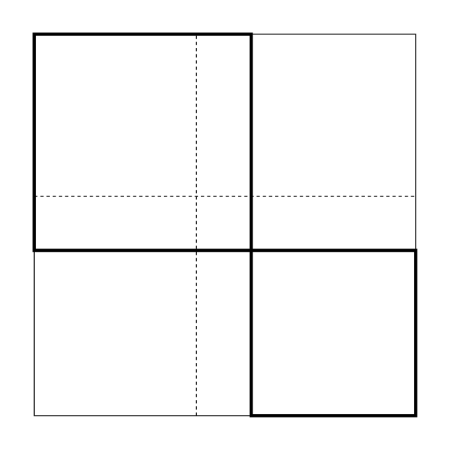
\(\square\left(c_{1}\right)+\square\left(c_{2}\right)=21^{\prime} 40^{\prime \prime} \quad, \quad c_{1}+c_{2}=50^{\prime}\).
Sin embargo, el autor elige un método diferente, mostrando así la flexibilidad de la técnica algebraica. Toma las dos áreas\(\square\left(c_{1}\right)\) y\(\square\left(c_{2}\right)\) como lados de un rectángulo, cuya área se puede encontrar haciendo\(10^{\prime}\) y\(10^{\prime}\) “sostener (Figura 4.10):
\(\square\left(c_{1}\right)+\square\left(c_{2}\right)=21^{\prime} 40^{\prime \prime}\),\(\left(\square\left(c_{1}\right), \square\left(c_{2}\right)\right)=10^{\prime} \times 10^{\prime}=1^{\prime} 40^{\prime \prime}\).


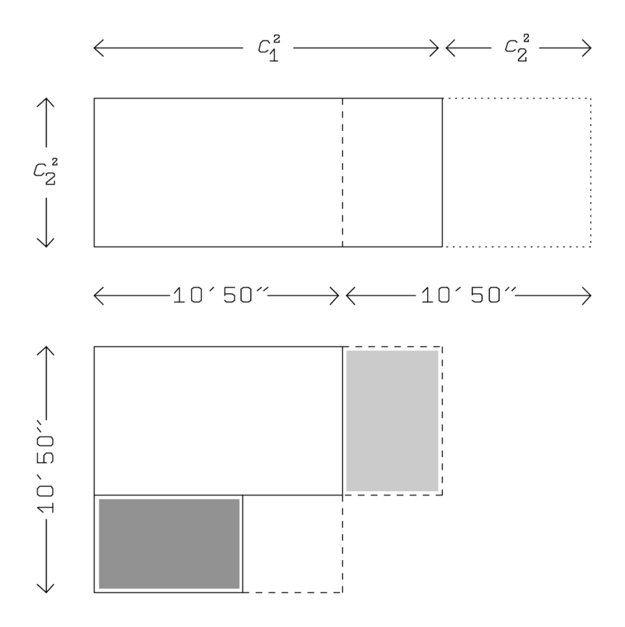
Lo que hay que tomar nota en este problema es de ahí que representa áreas por segmentos de línea y el cuadrado de un área por un área. Junto con las otras instancias de representación que hemos encontrado, el presente ejemplo nos permitirá caracterizar la técnica babilónica antigua como un álgebra genuina en la página 99.