9.2: Antiderivado

Has pasado muchas lecciones aprendiendo sobre cómo encontrar la derivada, f′ (x), de una función f (x), y el proceso de diferenciación. No debería sorprender entonces que hubiera un nombre para la función f (x), o familia de funciones, que pueda generar f′ (x) cuando se diferencie: f (x) y f′ (x) son un par de funciones inversas, y f (x) se llama antiderivada de f′ (x). Antes de continuar con la lección, ¿intenta enumerar funciones que son pares antiderivados y derivados?

---

El Antíderivado

Empecemos e introduzcamos la idea de la antiderivada de una función.

Una función F (x) se denomina antiderivada de una función f si F′ (x) =f (x) para todo x en el dominio de f.

¿Cómo se usa esta definición?

Considera la función$f(x)=3x^2 \nonumber$.

¿Se te ocurre una función F (x) tal que F′ (x) =f (x)? Deberías ser capaz de pensar en muchos de ellos.

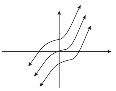
Ya que diferenciamos F (x) para obtener f (x), vemos que$F(x)=x^3+C \nonumber$ va a funcionar para cualquier constante C. Gráficamente, podemos pensar en el conjunto de todas las antiderivadas como transformaciones verticales de la gráfica de$F(x)=x^3 \nonumber$. La figura muestra dos transformaciones de este tipo.

CC BY-NC-SA

Con nuestra definición y ejemplo inicial, ahora buscamos formalizar la definición y desarrollar algunas reglas útiles con fines computacionales, y comenzar a ver algunas aplicaciones.

Introducción a Integrales Indefinidas

El proceso de búsqueda de antiderivados se denomina antidiferenciación, más comúnmente denominado integración. Así es como se indica la integración y cómo funciona:

F′ (x) =f (x)... Comienza con la ecuación diferencial que representa la definición de la antiderivada

$\int F′(x)dx=\int f(x)dx \nonumber$... Invoque la operación de integración (antidiferenciación) usando el símbolo especial ∫.

$F(x)+C= \int f(x)dx \nonumber$... Obtener el antiderivado F (x) y una constante de integración, C.

$\int f(x)dx=F(x)+C \nonumber$... Tenga en cuenta que si diferenciamos ambos lados, recuperamos la ecuación original:

$$\frac{d}{dx}[ \int f(x)dx]=f(x)=\frac{d}{dx}[F(x)+C]=F′(x) \nonumber$$

Nos referimos a f (x) dx como “la integral indefinida de f (x) con respecto a x”. La función f (x) se llama integrando y la constante C se llama la constante de integración . Finalmente el símbolo dx indica que vamos a integrar con respecto a x.

Usando esta notación, resumiremos el último ejemplo de la siguiente manera:

$$\int 3x^2dx=x^3+C \nonumber$$

Ahora, considere la función f (x) =cosx

¿Se te ocurre una función F (x) tal que F′ (x) =f (x)?

Si dijiste F (x) =SINX+C estarías en lo correcto y así es como se escribiría esto.

f (x) =F′ (x). Comienza con la ecuación diferencial que representa la definición de la antiderivada

COSx=F′ (x). Sustituto de f (x)

$\int cosx dx= \int F′(x)dx \nonumber$... Invoque la operación de integración (antidiferenciación) usando el símbolo especial ∫.

$\int cosx dx=F(x)+C \nonumber$... Obtener el antiderivado F (x) y una constante de integración, C.

$\int cosx dx=sinx+C \nonumber$... Sabemos F (x) =sinx porque si diferenciamos ambos lados, recuperamos la ecuación original.

Hemos visto las derivadas de una serie de funciones a través de los conceptos de cálculo y podemos armar una lista de funciones y sus antiderivadas como se muestra a continuación.

Resumen de Integrales Básicos Indefinidos Y Antiderivados

Función f (x)	Antiderivado$/int f(x)dx=F(x)+C \nonumber$
1	x+C
x	$\frac{x^2}{2}+C \nonumber$
$x^2 \nonumber$	$\frac{x^3}{3}+C \nonumber$
$x^n,\nonumber$ n−1	$\frac{x^{n+1}}{n+1}+C \nonumber$
$\frac{1}{x} \nonumber$	$lnx+C \nonumber$
sinx	−COSX+C
cosx	Sinx+C
$sec^2x \nonumber$	Tanx+C
$csc^2x \nonumber$	−CoTx+C
secxtanx	Secx+C
cscxcotx	−CSCX+C
$e^x \nonumber$	$e^x+C \nonumber$
$b^x \nonumber$ b>0	$\frac{b^x}{lnb}+C \nonumber$
$\frac{1}{xlnb} \nonumber$	$log_bx+C \nonumber$

Al igual que con la diferenciación, existen varias reglas para tratar la suma y diferencia de funciones integrables.

Reglas básicas de integración

Si f y g son funciones integrables, y C es una constante, entonces:

$$\int [f(x)+g(x)]dx= \int f(x)dx+ \int g(x)dx \nonumber$$ ,

$$\int [f(x)−g(x)]dx= \int f(x)dx− \int g(x)dx \nonumber$$ ,

$$\int [Cf(x)]dx=C \int f(x)dx \nonumber$$

Calcular la siguiente integral indefinida.

$$\int [2x^3+3x^2−1x]dx \nonumber$$

Usando nuestras reglas tenemos

$$\int [2x^3+3x^2−1x]dx=2 \int x^3dx+3 \int \frac{1}{x^2}dx− \int \frac{1}{x}dx \nonumber$$

$$=2(\frac{x^4}{4})+3(\frac{x^{−1}}{−1})−lnx+C \nonumber$$

$$=\frac{x^4}{2}−\frac{3}{x}−lnx+C \nonumber$$ .

Tenga en cuenta que a veces nuestras reglas necesitan ser modificadas ligeramente debido a operaciones con constantes.

---

Ejemplos

Ejemplo 1

Anteriormente, se le pidió que intentara enumerar funciones que son pares antiderivados y derivados. Al hacerlo estás presentando los resultados de las operaciones de diferenciación e integración. Si todo lo que hiciste fue enumerar la función que se está diferenciando como la antiderivada, esto es correcto. A estas alturas ya te has dado cuenta de que existe una familia de antiderivados entre los que podrías haber elegido, cada uno diferente por una constante de integración.

Ejemplo 2

Calcular la siguiente integral indefinida:

$$\int e^{3x}dx \nonumber$$ .

Primero notamos que nuestra regla para integrar funciones exponenciales no funciona aquí ya que ddxe3x=3e3x. Sin embargo, si recordamos dividir la función original por la constante entonces obtenemos la antiderivada correcta y tenemos

$$\int e^{3x}dx=\frac{e^{3x}}{3}+C \nonumber$$ .

Ahora podemos reafirmar la regla de una forma más general como

$$\int e^{kx}dx= \frac{e^{kx}}{3}+C \nonumber$$ .

---

Revisar

Para #1 -6, encuentra una antiderivada de la función

1. $f(x)=1−3x^2−6x \nonumber$
2. $f(x)=x−x^\{frac{2}{3}} \nonumber$
3. $f(x)=(2x+1)^{\frac{1}{5}} \nonumber$
4. $f(x)=cosx−x \nonumber$
5. $f(x)=x^5−7x^2+2 \nonumber$
6. $f(x)=e^{−2x}+e^x \nonumber$

Para #7 -12, encuentra la integral indefinida

7. \ (\ int (2+\ sqrt {5}) dx\ nonumber\]
8. $\int 2(x−3)^3dx \nonumber$
9. $\int (x^2⋅x^\frac{1}{3})dx \nonumber$
10. $\int (x+\frac{1}{x^4\sqrt{x}})dx \nonumber$
11. $(cosx+2sinx)dx \nonumber$
12. $\int 2sinxcosxdx \nonumber$
13. Resolver la ecuación diferencial$f′(x)=4x^3−3x^2+x−3 \nonumber$.
14. Encuentra la antiderivada F (x) de la función$f(x)=2e^{2x}+x−2 \nonumber$ que satisface F (0) =5.
15. Evaluar la integral indefinida$\int |x|dx \nonumber$ (Pista: Examinar la gráfica de f (x) =|x|.)

---

Reseña (Respuestas)

Para ver las respuestas de Revisar, abra este archivo PDF y busque la sección 5.1.

---

El vocabulario

Término	Definición
antiderivado	Un antiderivado es una función que invierte una derivada. La función A es la antiderivada de la función B si la función B es la derivada de la función A.
antidiferenciación	El proceso de búsqueda de antiderivados se denomina antidiferenciación, más comúnmente denominado integración.
constante de integración	La constante de integración es la constante C en la ecuación f (x) dx=F (x) +C relacionando la función f (x) y la antiderivada F.
integrand	Un integrando es el argumento f (x) en la integral indefinida f (x) dx.
integración	El proceso de búsqueda de antiderivados a veces se llama antidiferenciación, pero más comúnmente se conoce como integración.

---

Recursos adicionales

PLIX: Jugar, Aprender, Interactuar, EXPLORAR - Antiderivado: Reunirlo

Práctica: Antiderivado

Mundo real: Alto de las Montañas Rocosas