
3.3: Intervalos en E


- Última actualización
- 30 oct 2022
- Guardar como PDF

( \newcommand{\kernel}{\mathrm{null}\,}\)
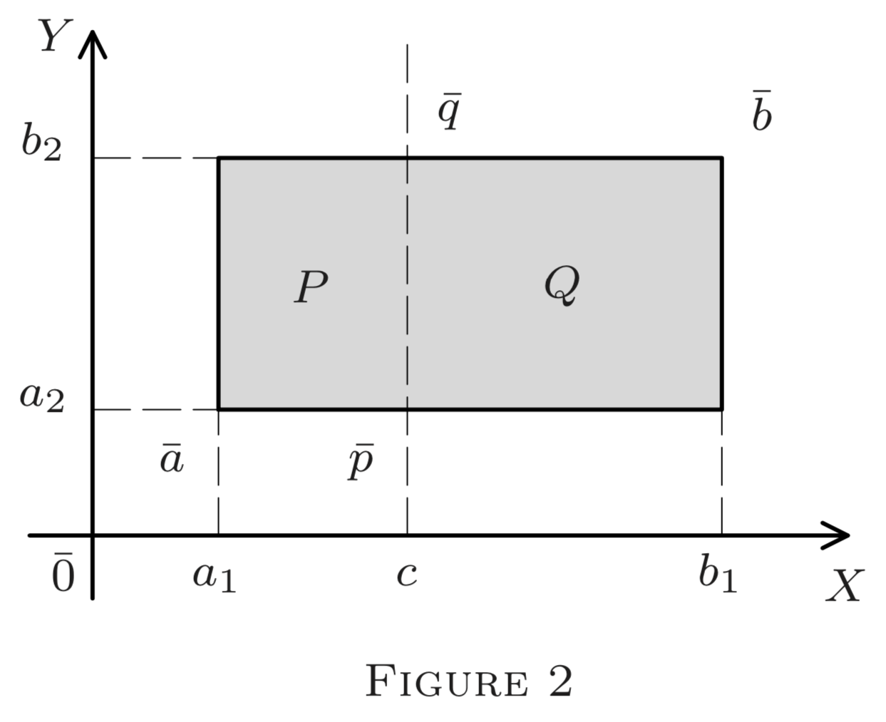
Considera el rectángulo queE2 se muestra en la Figura 2. Su interior (sin el perímetro consta de todos los puntos de(x,y)∈E2 tal manera que
a1<x<b1 and a2<y<b2;
es decir,
x∈(a1,b1) and y∈(a2,b2).
Así es el producto cartesiano de dos intervalos de línea,(a1,b1) y(a2,b2). Para incluir también todos o algunos lados, tendríamos que reemplazar los intervalos abiertos por los cerrados, semiterrados o medio abiertos. De igual manera, los productos cartesianos de tres intervalos de línea producen paralelepípedos rectangulares enE3. Llamamos a tales conjuntos enEn intervalos.
1. Por un intervalo enEn nos referimos al producto cartesiano de cualquiern intervalo enE1 (algunos pueden ser abiertos, algunos cerrados o semiabiertos, etc.).
2. En particular, dado
¯a=(a1,…,an) and ¯b=(b1,…,bn)
con
ak≤bk,k=1,2,…,n,
definimos el intervalo abierto(¯a,¯b), el intervalo cerrado[¯a,¯b], el intervalo medio abierto(¯a,¯b], y el intervalo semicerrado de la[¯a,¯b) siguiente manera:
(¯a,¯b)={¯x|ak<xk<bk,k=1,2,…,n}=(a1,b1)×(a2,b2)×⋯×(an,bn)[¯a,¯b]={¯x|ak≤xk≤bk,k=1,2,…,n}=[a1,b1]×[a2,b2]×⋯×[an,bn](¯a,¯b]={¯x|ak<xk≤bk,k=1,2,…,n}=(a1,b1]×(a2,b2]×⋯×(an,bn][a,b)={¯x|ak≤xk<bk,k=1,2,…,n}=[a1,b1)×[a2,b2)×⋯×[an,bn)
En todos los casos,¯a y se¯b denominan los puntos finales del intervalo. Su distancia
ρ(¯a,¯b)=|¯b−¯a|
se llama su diagonal. Lasn diferencias
bk−ak=ℓk(k=1,…,n)
se llaman susn longitudes de borde. Su producto
n∏k=1ℓk=n∏k=1(bk−ak)
se llama el volumen del intervalo (enE2 ella está su área, enE1 su longitud).\) El punto
¯c=12(¯a+¯b)
se llama su centro o punto medio. La diferencia establecida
[¯a,¯b]−(¯a,¯b)
se llama el límite de cualquier intervalo con puntos finales¯a y→b; consta de 2n “caras” definidas de manera natural. (¿Cómo?)
A menudo denotamos intervalos por letras simples, por ejemplo. A=(¯a,¯b),y escribirdA para “diagonal deA′′ yvA o volA para “volumen deA." Si todas las longitudes de bordebk−ak son iguales,A se llama un cubo (enE2, un cuadrado). ASe dice que el intervalo es degenerado iffbk=ak para algunosk, en cuyo caso, claramente,
volA=n∏k=1(bk−ak)=0.
Nota 1. Tenemos¯x∈(¯a,¯b) iff las desigualdades seak<xk<bk mantienen simultáneamente para todosk. Esto es imposible siak=bk para algunos dek; manera similar para las desigualdadesak<xk≤bk oak≤xk<bk. Así un intervalo degenerado está vacío, a menos que esté cerrado (en cuyo caso contiene¯a y al¯b menos).
Nota 2. En cualquier intervaloA,
dA=ρ(¯a,¯b)=√n∑k=1(bk−ak)2=√n∑k=1ℓ2k.
EnE2, podemos dividir un intervaloA en dos subintervalosP yQ dibujando una línea (ver Figura 2). EnE3, esto se hace por un plano ortogonal a uno de los ejes de la forma\boldsymbol{x_{k}=c\left(} ver §§4-6, Nota 2), conak<c<bk. En particular, si\ derecho. c=12(ak+bk),el plano bisecta el bordek th deA; y así la longitud del bordek th deP( y esQ) igual a12ℓk=12(bk−ak). SiA está cerrado, así esP oQ, dependiendo de nuestra elección. (Podemos incluir la “partición”xk=c enP oQ.)1
Ahora, sucesivamente dibujarn planosxk=ck,ck=12(ak+bk),k=1,2,…,n. El primer plano bisecaℓj dejando los otros bordes deAun− cambiado. Los dos subintervalos resultantesP yQ luego son cortados por el planox2=c2, bisectando el segundo borde en cada uno de ellos. Así obtenemos cuatro subintervalos (ver Figura 3 paraE2. Cada plano sucesivo duplica el número de subintervalos. Después den los pasos, obtenemos intervalos2n disjuntos, con todos los bordesℓk bisecados. Así por Nota2, la diagonal de cada uno de ellos es
√n∑k=1(12ℓk)2=12√n∑k=1ℓ2k=12dA.
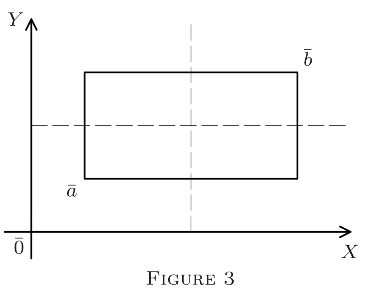
Nota 3. SiA se cierra entonces, como se señaló anteriormente, podemos hacer que cualquiera (pero sólo uno) de los2n subintervalos se cierre manipulando adecuadamente cada paso.
Se deja al lector la prueba de los siguientes corolarios simples.
Ninguna distancia entre dos puntos de un intervaloA superadA, su diagonal. Es decir,(∀¯x,¯y∈A)ρ(¯x,¯y)≤dA
Si un intervaloA contiene¯p y¯q, luego tambiénL[¯p,¯q]⊆A.
Cada intervalo no degenerado enEn contiene puntos racionales, es decir, puntos cuyas coordenadas son todas racionales.
(Pista: Utilice la densidad de los racionales enE1 para cada coordenada por separado.)